TensorFlow - Python Deep Learning Neural Network API

Train MobileNet using transfer learning

In this episode, we'll be training our fine-tuned MobileNet model on images from our own data set, and we'll also be evaluating the model by using it to predict on unseen images.

From the work we did together in the last episode, we now have a MobileNet model that has been built and tuned to be able to classify images of cats and dogs. We're now going to train the model, observe the results, and then we'll use the model for inference to evaluate how well the model predicts on images that it didn't see during training or validation.

Before we get started with the new code, make sure you have all the earlier code in place that we went through together in the previous episodes.

Training the model

We'll be working with the fine-tuned MobileNet model that we created last time and stored in the model variable.

model.compile(
      optimizer=Adam(learning_rate=0.0001)
    , loss='categorical_crossentropy'
    , metrics=['accuracy']
)

On this model, we're first calling compile and specifying the Adam optimizer with a learning rate of .0001. We're setting the loss to categorical_crossentropy, and our metrics just include accuracy.

After our model is compiled, we're now going to train the model by calling fit().

model.fit(
      x=train_batches
    , steps_per_epoch=len(train_batches)
    , validation_data=valid_batches
    , validation_steps=len(valid_batches)
    , epochs=10
    , verbose=2
)

To fit(), we pass our training set, which is stored in the train_batches directory iterator we created last time with a Keras ImageDataGenerator().

We also need to specify steps_per_epoch to indicate how many batches of samples from our training set should be passed to the model before declaring one epoch complete.

Next we set the validation_data parameter equal to our valid_batches variable. Similar to steps_per_epoch, we specify validation_steps in the same fashion but with using valid_batches.

Next, we specify the number of epochs to run, and we're going to go with 10. Finally, we set verbose equal to 2, which will print out an individual line with performance metrics for each epoch.

Running this code, we can see that after just 10 epochs, our model is performing extremely well on classifying cat and dog images.

Train for 100 steps, validate for 20 steps
Epoch 1/10
100/100 - 35s - loss: 0.2669 - accuracy: 0.8810 - val_loss: 0.0634 - val_accuracy: 0.9650
Epoch 2/10
100/100 - 3s - loss: 0.0808 - accuracy: 0.9730 - val_loss: 0.0476 - val_accuracy: 0.9800
Epoch 3/10
100/100 - 3s - loss: 0.0417 - accuracy: 0.9940 - val_loss: 0.0384 - val_accuracy: 0.9800
Epoch 4/10
100/100 - 3s - loss: 0.0221 - accuracy: 1.0000 - val_loss: 0.0284 - val_accuracy: 0.9800
Epoch 5/10
100/100 - 3s - loss: 0.0148 - accuracy: 1.0000 - val_loss: 0.0266 - val_accuracy: 0.9850
Epoch 6/10
100/100 - 3s - loss: 0.0111 - accuracy: 1.0000 - val_loss: 0.0320 - val_accuracy: 0.9850
Epoch 7/10
100/100 - 3s - loss: 0.0087 - accuracy: 1.0000 - val_loss: 0.0256 - val_accuracy: 0.9900
Epoch 8/10
100/100 - 3s - loss: 0.0070 - accuracy: 1.0000 - val_loss: 0.0281 - val_accuracy: 0.9850
Epoch 9/10
100/100 - 3s - loss: 0.0058 - accuracy: 1.0000 - val_loss: 0.0276 - val_accuracy: 0.9850
Epoch 10/10

With the minor tuning we did to the model last time, it is performing very well on this new task.

Using the model for inference

Next, we're going to use our model to predict on images from our test set that it hasn't already seen during training or validation.

Before we run the predictions, we're going to get and format the labels for the test set, and we need these just in order to plot the confusion matrix we'll see in a few moments. We don't actually need the labels to get predictions from the model.

First, we define test_labels to be equal to test_batches.classes.

test_labels = test_batches.classes

Recall, we defined test_batches in the last episode.

Calling classes on test_batches is going to give us the class names (i.e. the labels), for each sample in the test set. This is the reason we specified shuffle=False for test_batches in the last episode.

Since we'll be using these static labels that are returned from test_batches.classes, we can't shuffle our test data each time we use it for predicting because then the labels won't map correctly to the data.

By calling class_indices on test_batches, we can see the mapping from the underlying class names, cat and dog, to the 0s and 1s. The output of test_batches.class_indices looks like this.

{'cat': 0, 'dog': 1}

So, we can see that a cat label corresponds to 0, and a dog label corresponds to 1.

We've now got our labels taken care of. Let's now get some predictions.

predictions = model.predict(x=test_batches, verbose=0)

We define this predictions variable to be equal to model.predict(), and we're passing in our test_batches.

Lastly, we set the verbosity equal to 0, which is just not going to print out any output.

Once we run this code, and our predictions are finished, we need a way to visualize them, so we're going to plot them in a confusion matrix.

Visualize predictions in confusion matrix

We'll be using the scikit-learn library to do that. If you're not generally familiar with confusion matrices, or you want to learn more about working with them, check out the earlier episode where we go into more detail on using scikit-learn's confusion matrix.

First, we have a function called plot_confusion_matrix(), and this is what we'll be calling in a few moments to do the plotting.

def plot_confusion_matrix(cm, classes,
        normalize=False,
        title='Confusion matrix',
        cmap=plt.cm.Blues):
    """
    This function prints and plots the confusion matrix.
    Normalization can be applied by setting `normalize=True`.
    """
    plt.imshow(cm, interpolation='nearest', cmap=cmap)
    plt.title(title)
    plt.colorbar()
    tick_marks = np.arange(len(classes))
    plt.xticks(tick_marks, classes, rotation=45)
    plt.yticks(tick_marks, classes)

    if normalize:
        cm = cm.astype('float') / cm.sum(axis=1)[:, np.newaxis]
        print("Normalized confusion matrix")
    else:
        print('Confusion matrix, without normalization')

    print(cm)

    thresh = cm.max() / 2.
    for i, j in itertools.product(range(cm.shape[0]), range(cm.shape[1])):
        plt.text(j, i, cm[i, j],
            horizontalalignment="center",
            color="white" if cm[i, j] > thresh else "black")

    plt.tight_layout()
    plt.ylabel('True label')
    plt.xlabel('Predicted label')

Note that this code was pulled directly off of scikit-learn's website, so we're not going to go over the details here.

Next, we create this confusion_matrix object called cm, and we set it equal to scikit-learn's confusion_matrix that we imported at the start of our code in the last episode.

cm = confusion_matrix(y_true=test_labels, y_pred=predictions.argmax(axis=1))

To our confusion matrix, we pass the labels of our test set as well as the prediction results stored in predictions. Calling argmax on the predictions is going to return the indices that contain the maximum values from the list of predictions. So, because we only have two classes, it will return a 0 or 1 for each prediction in the predictions list.

Next, we define the labels for our confusion matrix, and these need to be in the order that the class indices are in. Recall the class indices from test_batches we checked out above.

cm_plot_labels = ['cat','dog']

Since cat was first and then dog in the class indices dictionary, that's how we specify the order for the confusion matrix labels.

Then, we call the plot_confusion_matrix() function that we referenced above, and we pass in our confusion matrix cm, the labels cm_plot_labels, and we give it the title of 'Confusion Matrix'.

plot_confusion_matrix(cm=cm, classes=cm_plot_labels, title='Confusion Matrix')

Running this line, we get this plot as a result.

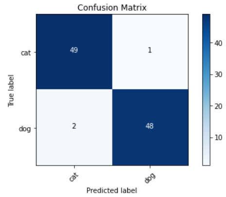
From analyzing the results from the confusion matrix, we can see that these predictions were pretty great with only incorrectly predicted 3 out of 100 samples.

We can conclude our fine-tuned model overall did a really great job on the task of classifying images as cats or dogs.

Next, we're going to build and fine-tune another MobileNet model, but this time, it's going to be on classes of images that weren't included in the ImageNet data set that the original MobileNet was trained on, so we'll likely need to do a bit more tuning. Stay tuned to see how that model holds up.

If you're following along with the code yourself, let me know in the comments how your MobileNet model is holding up to any fine-tuning that you're implementing, and I'll see ya in the next one!