Backpropagation Explained - Backprop Crash Course
Unlock the Secrets of Neural Network Training


Backpropagation in Neural Networks
Hey, what's going on everyone? Today, we delve into the world of backpropagation—the heart of the neural network training process.
Without further ado, let's dive in.
Stochastic Gradient Descent (SGD) Review
First things first: we highly recommend checking out our previous posts on training an artificial neural network and how a network learns if you haven't already. Done? Great, let's move on.
We'll kick off with a quick recap of stochastic gradient descent (SGD), and then focus on where backpropagation comes into play. The majority of our time will be spent unraveling the intuition behind backpropagation.
Previously, we touched on how SGD works to minimize the loss function by iteratively updating the weights during training. Now, it's time to delve deeper.
The crucial act of calculating gradients for weight updates is performed through a process called backpropagation.
Alright, let's set the stage for this discussion.
Forward Propagation
To keep things simple, let's consider a network with two hidden layers. For the sake of this explanation, we're dealing with a single sample of input.

As a refresher, data flows forward through the network—from input layer to output layer—in a process known as forward propagation.
Every node receives input from the previous layer, performs a weighted sum operation, passes it through an activation function, and sends the output to the next layer. This process continues until the data reaches the output layer.
Upon reaching the output layer, the model generates a prediction. In a classification task, such as identifying animals in images, the output node with the highest activation indicates the model's choice.
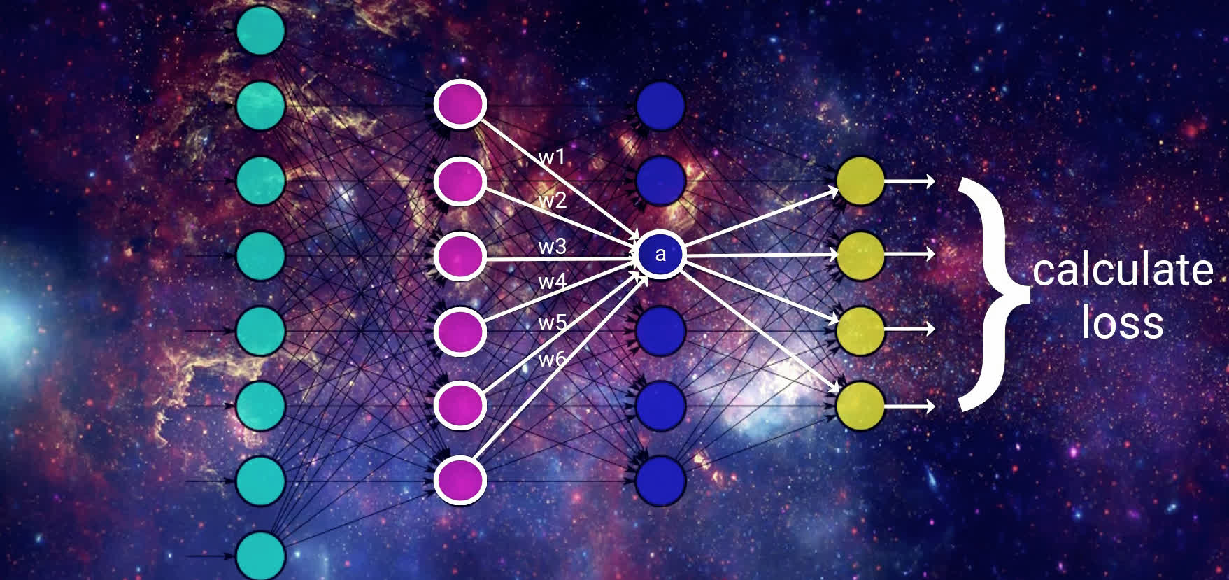
Calculating the Loss
Next, we compute the loss based on this prediction. The specific method depends on the loss function chosen, but generally, it measures how far off the model's prediction is from the actual value.
Now, here's where gradient descent steps in: its objective is to minimize this loss by updating the weights, and it does so using the calculated gradients.
\[\frac{d\left( loss\right) }{d\left( weight\right) }\]
This is where backpropagation enters the scene.
Having covered forward propagation, it's logical to infer that backpropagation means working in reverse. Starting from the output, where the loss has been calculated, we traverse back through the network to update the weights.
Now, let's concentrate on the core intuition behind backpropagation.
Intuitive Understanding of Backpropagation
To update the weights, gradient descent is going to start by looking at the activation outputs from our output nodes.
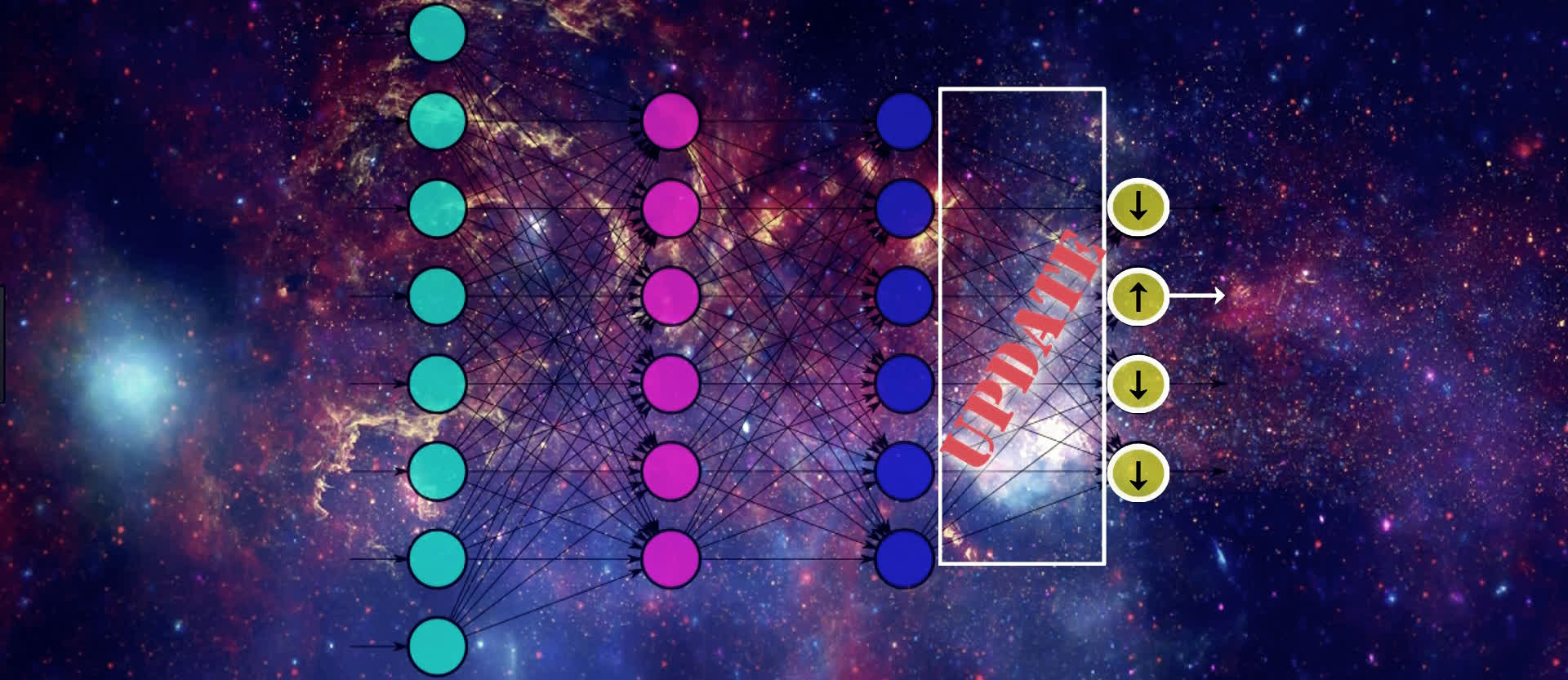
Suppose that this output node here with the up arrow pictured below maps to the output that our given input actually corresponds to. If that's the case, then gradient descent understands that the value of this output should increase, and the values from all the other output nodes should decrease. Doing this will help SGD lower the loss for this input.
We know that the values of these output nodes come from the weighted sum of the weights for the connections in the output layer here being multiplied by the output from the previous layer and then passing this weighted sum to the output layer's activation function.
Therefore, if we want to update the values for the output nodes in the way we just discussed, one way to do this is by updating the weights for these connections that are connected to the output layer. Another way of doing this is by changing the activation output from the previous layer.
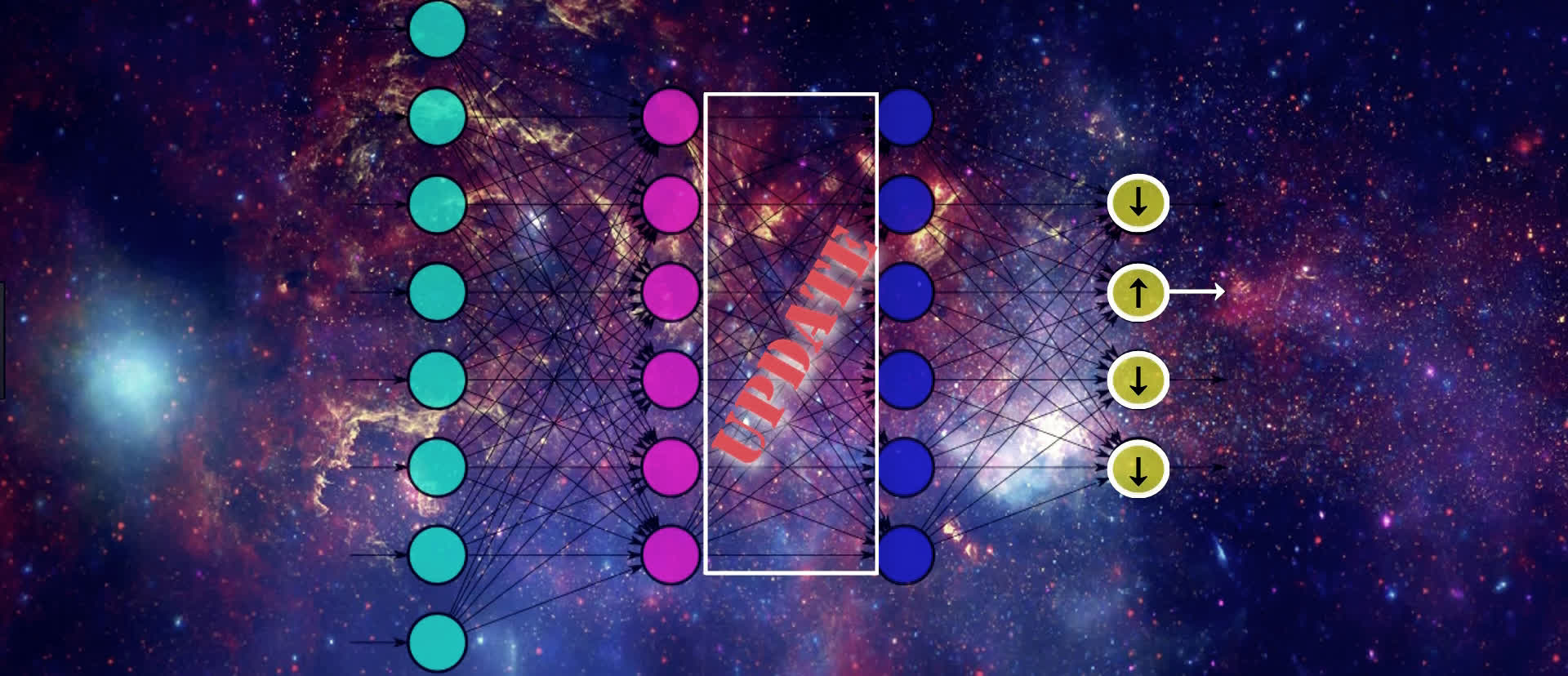
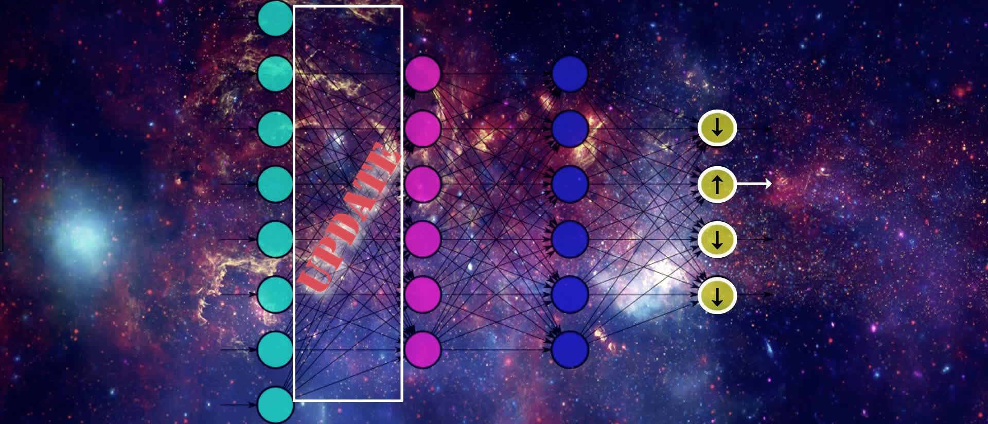
We can't actually directly change the activation output because it's a calculation based on the weights and the previous layer's output. But, we can indirectly influence a change in this layer's activation output by jumping backwards, and again, updating the weights here in the same way we just discussed for the output layer.
We continue this process until we reach the input layer. We don't want to change any of the values from the nodes in our input layer since this contains our actual input data.
As we can see, we're moving backwards through our network, updating the weights from right to left in order to slightly move the values from our output nodes in the direction that they should be going in order to help lower the loss.
This means that, for an individual sample, SGD is trying to increase the output value for the correct output node and decrease the output value for the incorrect output nodes, which, in turn, of course, decreases the loss.
It's also important to note, that in addition to updating weights to move in the desired direction i.e. positive or negative, backpropagation is also working to efficiently update the weights so that the updates are being done in a manner that helps to reduce the loss function most efficiently.
The proportion in which some weights are updated relative to others may be higher or lower, depending on how much affect the update is going to have on the network as a whole to lower the loss.
After calculating the derivatives, the weights are proportionally updated to their new values using the derivatives we obtain. The technical explanation for this update is shown in this lesson about how a neural network learns.
We went through this example for a single input, but this exact same process will occur for all the input for each batch we provide to our network, and the resulting updates to the weights in the network are going to be the average updates that are calculated for each individual input.
These averaged results for each weight are indeed the corresponding gradient of our loss function with respect to each weight.
Summary of this process
Alright, we've done a lot, so let's give a quick summary of it all. When training an artificial neural network, we pass data into our model. The way this data flows through the model is via forward propagation where we're repeatedly calculating the weighted sum of the previous layers activation output with the corresponding weights, and then passing this sum to the next layer's activation function.
We do this until we reach the output layer. At this point, we calculate the loss on our output, and gradient descent then works to minimize this loss.
Gradient descent does this minimization process by first calculating the gradient of the loss function and then updating the weights in the network accordingly. To do the actual calculation of the gradient, gradient descent uses backpropagation.
Ok, so this covers the intuition behind what backpropagation is doing, but of course, this is all done with math behind the scenes.
Calculus behind the scenes
The backpropagation process we just went through uses calculus. Recall, that backpropagation is working to calculate the derivative of the loss with respect to each weight.
To do this calculation, backprop is using the chain rule to calculate the gradient of the loss function. If you've taken a calculus course, then you may be familiar with the chain rule as being a method for calculating the derivative of the composition of two or more functions. We'll start covering the mathematics of this process in the next section.
At this point, we should now have a fuller picture for what's going on when we're training a neural network, where backpropagation fits into this process, and what the intuition is behind backpropagation.
Backprop Mathematical Notation
In this section, we're going to get started with the math that's used in backpropagation during the training of an artificial neural network.
Without further ado, let's get to it.
We've covered the intuition behind what backpropagation's role is during the training of an artificial neural network. Now, we're going to focus on the math that's underlying backprop.
Recapping backpropagation
Let's recap how backpropagation fits into the training process.
We know that after we forward propagate our data through our network, the network gives an output for that data. The loss is then calculated for that predicted output based on what the true value of the original data is.
Stochastic gradient descent, or SGD, has the objective to minimize this loss. To do this, it calculates the derivative of the loss with respect to each of the weights in the network. It then uses this derivative to update the weights.

It does this process over and over again until it's found a minimized loss. We covered how this update is actually done using the learning rate in our previous post that covers how a neural network learns.
When SGD calculates the derivative, it's doing this using backpropagation. Essentially, SGD is using backprop as a tool to calculate the derivative, or the gradient, of the loss function.
Going forward, this is going to be our focus. All the math that we'll be covering in the next few sections will be for the sole purpose of seeing how backpropagation calculates the gradient of the loss function with respect to the weights.
Ok, we've now got our refresher of backprop out of the way, so let's jump into to the math!
Backpropagation Mathematical Notation
As discussed, we're going to start out by going over the definitions and notation that we'll be using going forward to do our calculations.
This table describes the notation we'll be using throughout this process.
| Symbol | Definition |
|---|---|
| \(L\) | Number of layers in the network |
| \(l\) | Layer index |
| \(j\) | Node index for layer \(l\) |
| \(k\) | Node index for layer \(l-1\) |
| \(y_{j}\) | The value of node \(j\) in the output layer \(L\) for a single training sample |
| \(C_{0}\) | Loss function of the network for a single training sample |
| \(w_{j}^{(l)}\) | The vector of weights connecting all nodes in layer \(l-1\) to node \(j\) in layer \(l\) |
| \(w_{jk}^{(l)}\) | The weight that connects node \(k\) in layer \(l-1\) to node \(j\) in layer \(l\) |
| \(z_{j}^{(l)}\) | The input for node \(j\) in layer \(l\) |
| \(g^{(l)}\) | The activation function used for layer \(l\) |
| \(a_{j}^{(l)}\) | The activation output of node \(j\) in layer \(l\) |
Let's narrow in and discuss the indices used in these definitions a bit further.
Importance of indices
Recall at the top of the table, we covered the notation that we'd be using to index the layers and nodes within our network. All further definitions then depended on these indices.
| Symbol | Definition |
|---|---|
| \(l\) | Layer index |
| \(j\) | Node index for layer \(l\) |
| \(k\) | Node index for layer \(l-1\) |
We saw that, for each of the terms we introduced, we have either a subscript or a superscript, or both. Sometimes, our subscript even had two terms, as we saw when we defined the weight between two nodes.
These indices we're using everywhere may make the terms look a little intimidating and overly bulky. That's why I want to focus on this topic further here.
It turns out that if we use these indices properly and we understand their purpose, it's going to make our lives a lot easier going forward when working with these terms and will reduce any ambiguity or confusion, rather than induce it.
In code, when we run loops, like a for loop or a while loop that, the data that the loop is iterating over is an indexed sequence of data.
// pseudocode (java)
for (int i = 0; i < data.length; i++) {
    #do stuff
}
Indexed data allows the code to understand where to start, where to end, and where it is, at any given point in time, within the loop itself.
This idea of keeping track of where we are during an iteration over a sequence is precisely why keeping track of which layer, which node, which weight, or really, which anything that we introduced here, is important.
For the math in upcoming sections, we'll be seeing a lot of iteration, particularly via summation, where summation is simply the addition of a sequence of numbers. A summation is just the process of iterating over a sequence of values and summing them.
Math example:
Suppose that \((a_{n})\) is a sequence of numbers. The sum of this sequence is given by:
Code example:
Suppose that a = [1,2,3,4] is a sequence of numbers. The sum is given by:
int sum = 0;
while (j < a.length) {
    sum = sum + a[j];
}
Aside from iteration, any time we choose a specific item to work with, like a particular layer, node, or weight, the indexing that we introduced here is what will allow us to properly reference this particular item that we've chosen to focus on.
As it turns out, backpropagation itself is an iterative process, iterating backwards through each layer, calculating the derivative of the loss function with respect to each weight for each layer.
Given this, it should be clear why these indices are required in order to make sense of the math going forward. Hopefully, rather than causing confusion within our notation, these indices can instead become intuition for when we think about doing anything iterative over our network.
Wrapping up Notation
Alright, now we have all the mathematical notation and definitions we need for backprop going forward. At this point, take the time to make sure that you fully understand this notation and the definitions, and that you're comfortable with the indexing that we talked about. After you have this down, you'll be prepared to take the next step.

In the next section, we'll be using these definitions to make some mathematical observations regarding things that we already know about the training process.
These observations are going to be needed in order to progress to the relatively heavier math that comes into play when we start differentiating the loss function in order to calculate the gradient using backprop.
Mathematical Observations for Backpropagation
Hey, what's going on everyone? In this section, we're going to make mathematical observations about some facts we already know about the training process of an artificial neural network.
We'll then be using these observations going forward in our calculations for backpropagation. Let's get to it.
The path forward
In the last section, we focused on the mathematical notation and definitions that we would be using going forward to show how backpropagation mathematically works to calculate the gradient of the loss function.
Here, we're going to be making some mathematical observations about the training process of a neural network. The observations we'll be making are actually facts that we already know conceptually, but we'll now just be expressing them mathematically.
We'll be making these observations because the math for backprop that comes next, particularly, the differentiation of the loss function with respect to the weights, is going to make use of these observations.
We're first going to start out by making an observation regarding how we can mathematically express the loss function. We're then going to make observations around how we express the input and the output for any given node mathematically.
Lastly, we'll observe what method we'll be using to differentiate the loss function via backpropagation. Alright, let's begin.
Loss \(C_{0}\)
Observe that the expression
is the squared difference of the activation output and the desired output for node \(j\) in the output layer \(L\). This can be interpreted as the loss for node \(j\) in layer \(L\).
Therefore, to calculate the total loss, we should sum this squared difference for each node \(j\) in the output layer \(L\).
This is expressed as
Input \(z_{j}^{(l)}\)
We know that the input for node \(j\) in layer \(l\) is the weighted sum of the activation outputs from the previous layer \(l-1\).
An individual term from the sum looks like this:
So, the input for a given node \(j\) in layer \(l\) is expressed as
Activation Output \(a_{j}^{(l)}\)
We know that the activation output of a given node \(j\) in layer \(l\) is the result of passing the input, \(z_{j}^{\left( l\right) }\), to whatever activation function we choose to use \(g^{\left( l\right) }\).
Therefore, the activation output of node \(j\) in layer \(l\) is expressed as
\(C_{0}\) as a composition of functions
Recall the definition of \(C_{0}\),
So the loss of a single node \(j\) in the output layer \(L\) can be expressed as
We see that \(C_{0_{j}}\) is a function of the activation output of node \(j\) in layer \(L\), and so we can express \(C_{0_{j}}\) as a function of \(a_{j}^{\left( L\right) }\) as
Observe from the definition of \(C_{0_{j}}\) that \(C_{0_{j}}\) also depends on \( y_{j}\). Since \(y_{j}\) is a constant, we only observe \(C_{0_{j}}\) as a function of \(a_{j}^{\left( L\right) }\), and \(y_{j}\) as a parameter that helps define this function.
The activation output of node \(j\) in the output layer \(L\) is a function of the input for node \(j\). From an earlier observation, we know we can express this as
The input for node \(j\) is a function of all the weights connected to node \(j\). We can express \(z_{j}^{\left( L\right) }\) as a function of \(w_{j}^{\left( L\right) }\) as
Therefore,
Given this, we can see that \(C_{0}\) is a composition of functions.
We know that
and so using the same logic, we observe that the total loss of the network for a single input is also a composition of functions. This is useful in order to understand how to differentiate \(C_{0}\).
To differentiate a composition of functions, we use the chain rule.
Wrapping up Observations
Alright, so now we should understand the ways we can mathematically express the loss function of a neural network, as well as the input and the activation output of any given node.
Additionally, it should be clear now that the loss function is actually a composition of functions, and so to differentiate the loss with respect to the weights in the network, we'll need to use the chain rule.
Going forward, we'll be using the observations that we learned here in the relatively heavier math that we'll be using with backprop.
In the next section, we'll start getting exposure to this math. Before moving on to that though, take the time to make sure you understand these observations that we covered in this section and why we'll be working with the chain rule to differentiate the loss function.
Backpropagation Explained - Calculating the Gradient
In this section, we're finally going to see how backpropagation calculates the gradient of the loss function with respect to the weights in a neural network.
In the last section, we focused on how we can mathematically express certain facts about the training process.
Now we're going to be using these expressions to help us differentiate the loss of the neural network with respect to the weights.
Recall from the section that covered the intuition for backpropagation that for stochastic gradient descent to update the weights of the network, it first needs to calculate the gradient of the loss with respect to these weights.
Calculating this gradient is exactly what we'll be focusing on in this section.
We're first going to start out by checking out the equation that backprop uses to differentiate the loss with respect to weights in the network.
Then, we'll see that this equation is made up of multiple terms. This will allow us to break down and focus on each of these terms individually.
Lastly, we'll take the results from each term and combine them to obtain the final result, which will be the gradient of the loss function.
Alright, let's begin.
Derivative of the Loss Function with Respect to the Weights
Let's look at a single weight that connects node \(2\) in layer \(L-1\) to node \(1\) in layer \(L\).
This weight is denoted as
The derivative of the loss \( C_{0} \) with respect to this particular weight \( w_{12}^{(L)} \) is denoted as
Since \( C_{0} \) depends on \( a_{1}^{\left( L\right) }\text{,} \) and \( a_{1}^{\left( L\right) } \) depends on \( z_{1}^{(L)}\text{,}\) and \( z_{1}^{(L)} \) depends on \( w_{12}^{(L)}\text{,} \) the chain rule tells us that to differentiate \( C_{0} \) with respect to \( w_{12}^{(L)}\text{,} \) we take the product of the derivatives of the composed function.
This is expressed as
Let's break down each term from the expression on the right hand side of the above equation.
The first term: \( \frac{\partial C_{0}}{\partial a_{1}^{(L)}} \)
We know that
Therefore,
Expanding the sum, we see
Observe that the loss from the network for a single input sample will respond to a small change in the activation output from node \( 1 \) in layer \( L \) by an amount equal to two times the difference of the activation output \(a_{1}\) for node \( 1 \) and the desired output \( y_{1} \) for node \( 1 \).
The second term: \( \frac{\partial a_{1}^{(L)}}{\partial z_{1}^{(L)}} \)
We know that for each node \( j \) in the output layer \( L \), we have
and since \( j=1 \), we have
Therefore,
Therefore, this is just the direct derivative of \( a_{1}^{(L)} \) since \( a_{1}^{(L)} \) is a direct function of \( z_{1}^{\left(L\right)} \).
The third term: \( \frac{\partial z_{1}^{(L)}}{\partial w_{12}^{(L)}} \)
We know that, for each node \( j \) in the output layer \( L \), we have
Since \( j=1 \), we have
Therefore,
Expanding the sum, we see
The input for node \( 1 \) in layer \( L \) will respond to a change in the weight \( w_{12}^{(L)} \) by an amount equal to the activation output for node \( 2 \) in the previous layer, \( L-1 \).
Combining terms
Combining all terms, we have
We've seen how to calculate the derivative of the loss with respect to one individual weight for one individual training sample.
To calculate the derivative of the loss with respect to this same particular weight, \( w_{12} \), for all \( n \) training samples, we calculate the average derivative of the loss function over all \( n \) training samples.
This can be expressed as
We would then do this same process for each weight in the network to calculate the derivative of \( C \) with respect to each weight.
Wrapping Up Calculating the Gradient
At this point, we should now understand mathematically how backpropagation calculates the gradient of the loss with respect to the weights in the network.
We should also have a solid grip on all of the intermediate steps needed to do this calculation, and we should now be able to generalize the result we obtained for a single weight and a single sample to all the weights in the network for all training samples.
Now, we still haven't hit the point completely home by discussing the math that underlies the backwards movement of backpropagation that we discussed whenever we covered the intuition for backpropagation. Don't worry, we'll be doing that in the next section.
What puts the "back" in backprop?
In this section, we'll see the math that explains how backpropagation works backwards through a neural network.
Without further ado, let's get to it.
Setting Things Up
Alright, we've seen how to calculate the gradient of the loss function using backpropagation in the previous sections. We haven't yet seen though where the backwards movement comes into play that we talked about when we discussed the intuition for backprop.
Now, we're going to build on the knowledge that we've already developed to understand what exactly puts the back in backpropagation.
The explanation we'll give for this will be math-based, so we're first going to start out by exploring the motivation needed for us to understand the calculations we'll be working through.
We'll then jump right into the calculations, which we'll see, are actually quite similar to ones we've worked through in the previous sections.
After we've got the math down, we'll then bring everything together to achieve the mind-blowing realization for how these calculations are mathematically done in a backwards fashion.
Alright, let's begin.
Motivation
We left off from our last section by seeing how we can calculate the gradient of the loss function with respect to any weight in the network. When we went through the process for showing how that was calculated, recall that, we worked with this single weight in the output layer of the network.
Then, we generalized the result we obtained by saying this same process could be applied for all the other weights in the network.
For this particular weight, we saw that the derivative of the loss with respect to this weight was equal to this
Now, what would happen if we chose to work with a weight that is not in the output layer, like this weight here?
Well, using the formula we obtained for calculating the gradient of the loss, we see that the gradient of the loss with respect to this particular weight is equal to this
Alright, check it out. This equation looks just like the equation we used for the previous weight we were working with.
The only difference is that the superscripts are different because now we're working with a weight in the third layer, which we're denoting as \(L-1\), and then the subscripts are different as well because we're working with the weight that connects the second node in the second layer to the second node in the third layer.
Given this is the same formula, then we should just be able to calculate it in the exact same way we did for the previous weight we worked with in the last section, right?
Well, not so fast.
So yes, this is the same formula, and in fact, the second and third terms on the right hand side will be calculated using the same exact approach as we used before.
The first term on the right hand side of the equation is the derivative of the loss with respect to this one activation output, and for this one, there's actually a different approach required for us to calculate it.
Let's think about why.
When we calculated the derivative of the loss with respect to a weight in the output layer, we saw that the first term is the derivative of the loss with respect to the activation output for a node in the output layer.
Well, as we've talked about before, the loss is a direct function of the activation output of all the nodes in the output layer. You know, because the loss is the sum of the squared errors between the actual labels of the data and the activation output of the nodes in the output layer.
Ok, so, now when we calculate the derivative of the loss with respect a weight in layer \(L-1\), for example, the first term is the derivative of the loss with respect to the activation output for node two, not in the output layer, \(L\), but in layer \(L-1\).
And, unlike the activation output for the nodes in the output layer, the loss is not a direct function of this output.
See, because consider where this activation output is within the network, and then consider where the loss is calculated at the end of the network. We can see that the output is not being passed directly to the loss.
What we need now is to understand how to calculate this first term then. That's going to be our focus here.
If needed, go back and look at the previous section where we calculated the first term in the first equation to see the approach we took.
Then, use that information to compare with the approach we're going to use to calculate the first term in second equation.
| Which | Equation |
|---|---|
| First |
\[ \frac{\partial C_{0}}{\partial w_{12}^{(L)}} = \left(\frac{\partial C_{0}}{\partial a_{1}^{(L)}} \right) \left(\frac{\partial a_{1}^{(L)}}{\partial z_{1}^{(L)}} \right) \left(\frac{\partial z_{1}^{(L)}}{\partial w_{12}^{(L)}}\right) \]
|
| Second |
\[ \frac{\partial C_{0}}{\partial w_{22}^{(L-1)}} = \left( \frac{\partial C_{0}}{\partial a_{2}^{(L-1)}}\right) \left( \frac{\partial a_{2}^{(L-1)}}{\partial z_{2}^{(L-1)}}\right) \left( \frac{\partial z_{2}^{(L-1)}}{\partial w_{22}^{(L-1)}}\right) \]
|
Now, because the second and third terms on the right hand side of the second equation are calculated in the exact same manner as we've seen before, we're not going to cover those here.
We're just going to focus on how to calculate the first term on the right hand side of the second equation, and then we'll combine the results from all terms to see the final result.
Alright, at this point, go ahead and admit, you're thinking to yourself:
I hear you. We're getting there, so stick with me. We have to go through the math first and see what it's doing, and then once we see that, we'll be able to clearly see the whole point of the backwards movement.
So let's go ahead and jump in to the calculations.
Calculations
Alright, time to get set up.
We're going to show how we can calculate the derivative of the loss function with respect to the activation output for any node that is not in the output layer. We're going to work with a single activation output to illustrate this.
Particularly, we'll be working with the activation output for node \(2\) in layer \(L-1\).
This is denoted as
and the partial derivative of the loss with respect to this activation output is denoted as this
Observe that, for each node \(j\) in \(L\), the loss \(C_{0}\) depends on on \(a_{j}^{\left( L\right) }\), and \(a_{j}^{\left(L\right) }\) depends on \(z_{j}^{(L)}\). The node \(z_{j}^{(L)}\) depends on all of the weights connected to node \(j\) from the previous layer, \(L-1\), as well as all the activation outputs from \(L-1\).
This means that the node, \(z_{j}^{\left( L\right) }\) depends on \(a_{2}^{(L-1)}\).
Ok, now the activation output for each of these nodes depends on the input to each of these nodes.
In turn, the input to each of these nodes depends on the weights connected to each of these nodes from the previous layer, \(L-1\), as well as the activation outputs from the previous layer.
Given this, we can see how the input to each node in the output layer is dependent on the activation output that we've chosen to work with, the activation output for node \(2\) in layer \(L-1\).
Using similar logic to what we used in the previous section, we can see from these dependencies that the loss function is actually a composition of functions, and so, to calculate the derivative of the loss with respect to the activation output we're working with, we'll need to use the chain rule.
The chain rule tells us that to differentiate \(C_{0}\) with respect to \(a_{2}^{(L-1)}\), we take the product of the derivatives of the composed function. This derivative can be expressed as
This tells us that the derivative of the loss with respect to the activation output for node \(2\) in layer \(L-1\) is equal to the expression on the right hand side of the above equation.
This is the sum for each node \(j\) in the output layer, \(L\), of the derivative of the loss with respect to the activation output for node \(j\), times the derivative of the activation output for node \(j\) with respect to the input for node \(j\), times the input for node \(j\) with respect to the activation output for node \(2\) in layer \(L-1\).
Now, actually, this equation looks almost identical to the equation we obtained in the last section for the derivative of the loss with respect to a given weight. Recall that this previous derivative with respect to a given weight that we worked with was expressed as
Just eye-balling the general likeness between these two equations, we see that the only differences are one, the presence of the summation operation in our new equation, and two, the last term on the right hand side differs.
The reason for the summation is due to the fact that a change in one activation output in the previous layer is going to affect the input for each node \(j\) in the following layer \(L\), so we need to sum up these effects.
Now, we can see that the first and second terms on the right hand side of the equation are the same as the first and second terms in the last equation with regards to \(w_{12}^{\left( L\right) }\) in the output layer when \(j=1\).
Since we've already gone through the work to find how to calculate these two derivatives in the last section, we won't do it again here.
We're only going to focus on breaking down the third term, and then we'll combine all terms to see the final result.
The Third Term
Alright, so let's jump in to how to calculate the third term from the equation we just looked at.
The third term is the derivative of the input to any node \(j\) in the output layer \(L\) with respect to the activation output for node \(2\) in layer \(L-1\).
We know for each node \(j\) in layer \(L\) that
Therefore, we can substitute this expression in for \(z_{j}^{(L)}\) in our derivative.
Expanding the sum, we have
Due to the linearity of the summation operation, we can pull the derivative operator through to each term since the derivative of a sum is equal to the sum of the derivatives.
This means we're taking the derivatives of each of these terms with respect to \(a_{2}^{(L-1)}\), but actually we can see that only one of these terms contain \(a_{2}^{(L-1)}\).
This means that when we take the derivative of the other terms that don't contain \(a_{2}^{(L-1)}\), these terms will evaluate to zero.
Now taking the derivative of this one term that does contain \(a_{2}^{(L-1)}\), we apply the power rule, to obtain the result.
This result says that the input for any node \(j\) in layer \(L\) will respond to a change in the activation output for node \(2\) in layer \(L-1\) by an amount equal to the weight connecting node \(2\) in layer \(L-1\) to node \(j\) in layer \(L\).
Alright, let's now take this result and combine it with our other terms to see what we get as the total result for the derivative of the loss with respect to this activation output.
Combining the Terms
Alright, so we have our original equation here for the derivative of the loss with respect to the activation output we've chosen to work with.
From the previous section, we already know what these first two terms evaluate to. So I've gone ahead and plugged in those results, and since we have just seen what the result of the third term is, we plug it in as well.
Ok, so we've got this full result. Now what was it that we wanted to do with it again?
Oh yeah, now we can use this result to calculate the gradient of the loss with respect to any weight connected to node \(2\) in layer \(L-1\), like we saw for \(w_{22}^{(L-1)}\), for example, with the following equation
The result we just obtained for the derivative of the loss with respect to the activation output for node \(2\) in layer \(L-1\) can then be substituted for the first term in this equation.
As mentioned earlier, the second and third terms are calculated using the exact same approach we took for those terms in the previous section.
Notice that we've used the chain rule twice now. With one of those times being nested inside the other. We first used the chain rule to obtain the result for this entire derivative for the loss with respect to the given weight.
Then, we used it again to calculate the first term within this derivative, which itself was the derivative of the loss with respect to this activation output.
The results from each of these derivatives using the chain rule depended on derivatives with respect to components that reside later in the network.
Essentially, we're needing to calculate derivatives that depend on components later in the network first and then use these derivatives in our calculations of the gradient of the loss with respect to weights that come earlier in the network.
We achieve this by repeatedly applying the chain rule in a backwards fashion.
Average Derivative of the Loss Function
Note, to find the derivative of the loss function with respect to this same particular activation output, \(a_{2}^{(L-1)}\), for all \(n\) training samples, we calculate the average derivative of the loss function over all \(n\) training samples. This can be expressed as
Concluding Thoughts
Whew! Alright, now that we know what puts the back in backprop, we should now have a full understanding for what backprop is all about.