
TensorFlow.js - Examining tensors with the debugger
text
Using the debugger to examine tensors
What's up, guys? In this video, we're going to continue our exploration of tensors.
Here, we'll be stepping through the code we developed last time with the debugger to see the exact transformations that are happening to our tensors in real-time, so let's get to it.

Last time, we went through the process of writing the code to preprocess images for VGG16. Through that process, we gained exposure to working with tensors, transforming and manipulating them.
We're going to now step through these tensor operations with the debugger so we can see these transformations occur in real-time as we interact with our web app.
If you're not already familiar with using a debugger, don't worry, you'll still be able to follow.
We'll first go through this process using the debugger in Visual Studio code. Then, we'll demo the same process using the debugger built into the Chrome browser.
Starting the debugger
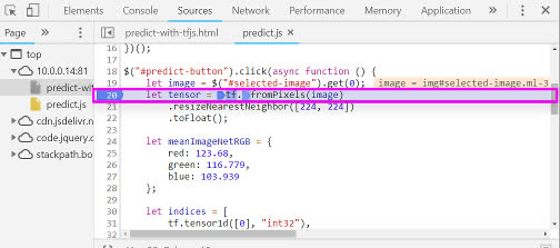
We're in our predict.js file within the click() event for the predict-button where all of our preprocessing code is written.
We're placing a breakpoint in our code where our first tensor is defined. Remember, this is where we're getting the selected image and transforming it into a tensor using tf.browser.fromPixels().
let tensor = tf.browser.fromPixels(image)
    .resizeNearestNeighbor([224, 224])
    .toFloat();
The expectation around this breakpoint is, when we browse to our app, the model will load, we'll select an image, and click the predict button. Once we click predict, the click() event
we'll be triggered, and we'll hit this breakpoint.
When this happens, the code execution will be paused until we tell it to continue to the next step. This means that while we're paused, we can inspect the tensors we're working with and see how they look before and after any given operation.
Let's see.
Let's start the debugger in the top left of the window, which will launch our app in Chrome.
We can see our model is loading.
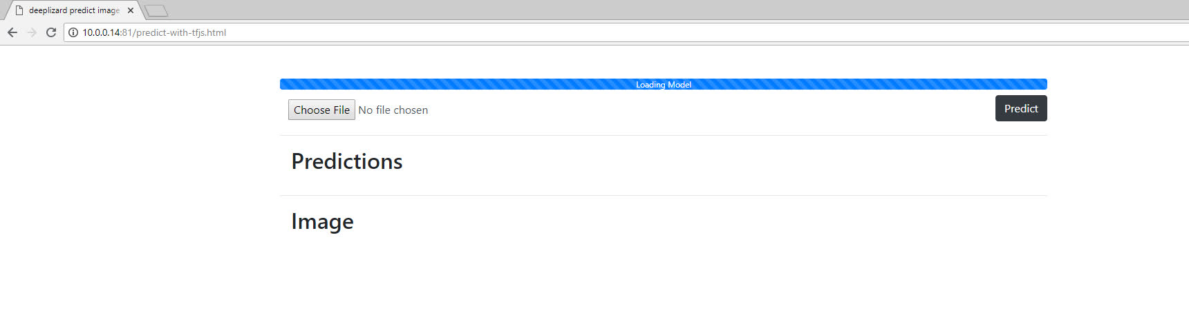
Ok, the model is loaded. Let's select an image and click the predict button. When we do this we'll see our breakpoint will get hit, and the app will pause.
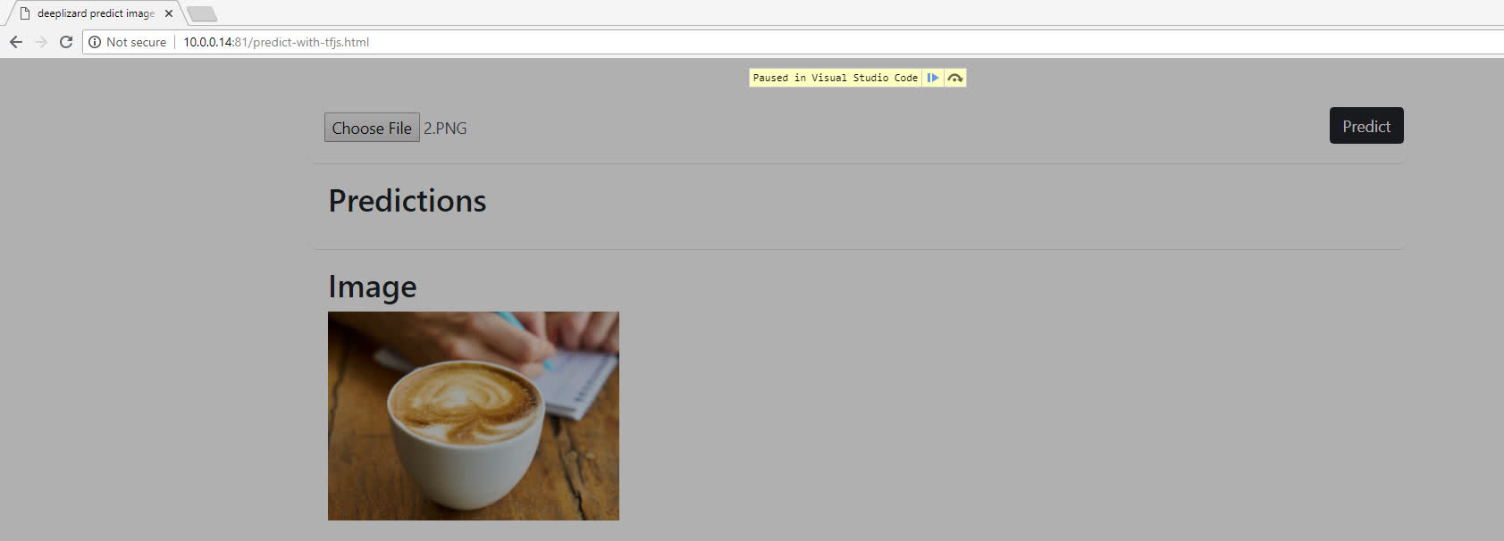
And here we go, our code execution is now paused.
Using the debugger
We're currently paused at this line where we define our Tensor object.
let tensor = tf.browser.fromPixels(image)
    .resizeNearestNeighbor([224, 224])
    .toFloat();
We're going to click the step-over icon, which will execute this code where we're defining tensor and will pause at the next step. Let's see.
Alright, we're now paused at the next step.
Now that tensor has been defined, let's inspect it a bit.
The Variables panel
First, we have this Variables panel where we can check out information about the variables in our app, and we can see our tensor variable is here in this list.
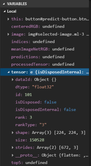
Clicking tensor, we can see all types of information about this object. For example, we can see the dtype is float32. The tensor is of rank-3. The shape is 224 x 224
x 3. The size is 150,528.
The debug console
Additionally, in the debug console we can play with this tensor further.
For example, let's print it using the TensorFlow.js print() function. This let's us get a printed summary of the data contained in this tensor.
> tensor.print()
Tensor
[[[56 , 29 , 4],
[58 , 30 , 3  ],
[59 , 30 , 3  ],
...,
[213, 183, 163],
[203, 170, 150],
[190, 153, 133]],

[[56 , 29 , 4  ],
[58 , 30 , 3  ],
[59 , 30 , 3  ],
...,
[213, 183, 163],
[203, 170, 150],
[190, 153, 133]],

[[53 , 27 , 5  ],
[55 , 28 , 4  ],
[57 , 29 , 4  ],
...,
[209, 178, 159],
[198, 162, 142],
[182, 143, 124]],

...

[[146, 98 , 39 ],
[143, 96 , 40 ],
[130, 86 , 36 ],
...,
[182, 130, 64 ],
[173, 123, 62 ],
[174, 123, 65 ]],

[[142, 94 , 34 ],
[139, 93 , 39 ],
[135, 92 , 43 ],
...,
[181, 127, 61 ],
[173, 121, 55 ],
[174, 122, 58 ]],

[[141, 93 , 38 ],
[133, 87 , 40 ],
[128, 85 , 38 ],
...,
[184, 130, 61 ],
[183, 129, 61 ],
[184, 130, 63 ]]]
Remember, we made this tensor have shape 224 x 224 x 3, so looking at this output, we can visualize this tensor as an object with 224 rows, each of which is 224 pixels across, and each of those pixels contains a red, green, and blue value.
So what's displayed here represents one of those 224 rows:
[[56 , 29 , 4 ],
[58 , 30 , 3  ],
[59 , 30 , 3  ],
...,
[213, 183, 163],
[203, 170, 150],
[190, 153, 133]]
The below represents one of the 224 pixels in this row, and each of these pixels contains first a red value, then a green value, then a blue value.
[56 , 29 , 4 ]
So, make sure you have a good grip on this idea so you can follow all the transformations this tensor is about to go through.
Stepping through the code
Alright, our debugger is paused on defining the meanImageNetRGB object. Let's go ahead and step over this so that it gets defined.
let meanImageNetRGB = {
    red: 123.68,
    green: 116.779,
    blue: 103.939
};
Again, we can now inspect this object over in the local variables panel. We're not doing any tensor operations here, so let's go ahead and move on.
We're now paused on our list of rank-1 tensors called indices, which we make use of later, so let's execute this.
let indices = [
    tf.tensor1d([0], "int32"),
    tf.tensor1d([1], "int32"),
    tf.tensor1d([2], "int32")
];
We can see indices now shows up in our Variables panel. Let's inspect this one a bit from the debug console.
If we just print out the list using console.log(indices), we get back that this is an array with three things in it. We know that each element in this array is a tensor, so let's access
one of them. Let's print the first tensor.
> indices[0].print()
Tensor
[0]
We get back that this object is a tensor, and we can see what it looks like. Just a one dimensional tensor with the single value zero. We can easily do the same thing for the second and third elements in the list too.
Inspecting tensor operations
We're now paused where we're defining the centeredRGB object, and from last time, we know that's where the bulk of our tensor operations are occurring.
let centeredRGB = {
    red: tf.gather(tensor, indices[0], 2)
        .sub(tf.scalar(meanImageNetRGB.red))
        .reshape([50176]),
    green: tf.gather(tensor, indices[1], 2)
        .sub(tf.scalar(meanImageNetRGB.green))
        .reshape([50176]),
    blue: tf.gather(tensor, indices[2], 2)
        .sub(tf.scalar(meanImageNetRGB.blue))
        .reshape([50176])
};
Alright, now, if we execute this block, then we'll skip over being able to inspect each of these transformations. So what we'll do is stay paused here, but in the console, we'll mimic each of these individual transformations one-by-one so we can see the before and after version of the tensor.
So, for example, we're first going to mimic what's happening here with the creation of the tensor that contains all the centered red values within our centeredRGB object.
In the console, we'll create a variable called red and set it equal to just this first call to tf.gather() and see what it looks like.
> red = tf.gather(tensor, indices[0], 2)
Before we do any of the other operations, let's see what this looks like. Let's first check the shape.
> red.shape
Array(3) [224, 224, 1]
Okay, 224 x 224 x 1. So, that's similar what we saw from the original tensor of 224 x 224 x 3, but rather than the last dimension containing all three pixel values, red, green, and blue, our new red tensor only contains the red pixel values.
Let's print red.
> red.print()
Tensor
[[[56 ],
[58 ],
[59 ],
...,
[213],
[203],
[190]],
[[56 ],
[58 ],
[59 ],
...,
[213],
[203],
[190]],
[[53 ],
[55 ],
[57 ],
...,
[209],
[198],
[182]],
...
[[146],
[143],
[130],
...,
[182],
[173],
[174]],
[[142],
[139],
[135],
...,
[181],
[173],
[174]],
[[141],
[133],
[128],
...,
[184],
[183],
[184]]]
Just to hit the point home, let's compare this to the original tensor. So the first three values in red are 56, 58, 59. Let's now check out the original tensor to see if this lines up.
Scrolling back up to the original tensor, we see it has the red values of 56, 58, and 59 in the first three zeroth indices along the second axis. So, red is just made up of each of these red
values.
Ok, let's see what the next operation on red is.
This is where we're centering each red value by subtracting the mean red value from ImageNet using the sub() function. Let's make a new variable called centeredRed and mimic this operation.
> centeredRed = red.sub(tf.scalar(meanImageNetRGB.red))
And now let's print the centeredRed tensor.
> centeredRed.print()
Tensor
[[[-67.6800003 ],
    [-65.6800003 ],
    [-64.6800003 ],
    ...,
    [89.3199997  ],
    [79.3199997  ],
    [66.3199997  ]],

    [[-67.6800003 ],
    [-65.6800003 ],
    [-64.6800003 ],
    ...,
    [89.3199997  ],
    [79.3199997  ],
    [66.3199997  ]],

    [[-70.6800003 ],
    [-68.6800003 ],
    [-66.6800003 ],
    ...,
    [85.3199997  ],
    [74.3199997  ],
    [58.3199997  ]],

    ...
    [[22.3199997  ],
    [19.3199997  ],
    [6.3199997   ],
    ...,
    [58.3199997  ],
    [49.3199997  ],
    [50.3199997  ]],

    [[18.3199997  ],
    [15.3199997  ],
    [11.3199997  ],
    ...,
    [57.3199997  ],
    [49.3199997  ],
    [50.3199997  ]],

    [[17.3199997  ],
    [9.3199997   ],
    [4.3199997   ],
    ...,
    [60.3199997  ],
    [59.3199997  ],
    [60.3199997  ]]]
Ok, -67.68, -65.68, and -64.68 are the first three values along the second axis. Let's compare this to the original red tensor now.
Scrolling up to the print out of the original red tensor, we see the first three values are 56, 58, and 59.
So, if we do the quick math of subtracting the mean red value of 123.68 from these first three values of red, we do indeed end up with the centered values of -67.68, -65.68, and -64.68 in the
new centeredRed tensor.
Now, centeredRed still has the same shape as red, which recall was 224 x 224 x 1. The next step is to reshape this tensor to be a rank-1 tensor of size 50,176. So we just want to
bring all the centered red values together, which are currently each residing in their own individual tensors.
So, to mimic this reshape() call, we'll make a new variable called reshapedRed.
> reshapedRed = centeredRed.reshape([50176])
Alright, let's check the shape to get confirmation.
> reshapedRed.shape
Array(1) [50176]
We see it is indeed the shape we specified. Let's now look at the print out of reshapedRed.
> reshapedRed.print()
Tensor
[-67.6800003, -65.6800003, -64.6800003, ..., 60.3199997, 59.3199997, 60.3199997]
We see that all the red values are now listed out in a one dimensional tensor.
Alright, so that's it for getting all the centered red values. As mentioned last time, we go through the same process to gather all the blues and greens as well, so we're not going to go through that in the debugger.
We'll now execute this block of code to create this centeredRGB object and move onto the next step.
This is where we're bringing our centered red, green and blue values all together into a new, processed tensor.
let processedTensor = tf.stack([centeredRGB.red, centeredRGB.green,
    centeredRGB.blue], 1)
    .reshape([224, 224, 3])
    .reverse(2)
    .expandDims();
So from the console, let's run this first tf.stack() operation by creating a variable called stackedTensor.
> stackedTensor = tf.stack([centeredRGB.red, centeredRGB.green, centeredRGB.blue], 1)
Remember, we just saw that the reshapedRed tensor ended up being a rank-1 tensor of shape 50,176. The green and blue tensors have the same shape and size, so when we stack them along axis one,
we should now have a 50,176 x 3 tensor.
You make think the result of the stack operation would look like this, where we have the centeredRed tensor with its 50,176 values stacked on top of the green tensor stacked on top of the blue
tensor.
And that's how it would look if we were stacking along axis zero. Because we're stacking along axis one though, we will get something that looks like this where we have 50,176 rows, each of which is made up of a single pixel with a red, green, and blue value.
Let's check the shape now in the console to be sure we get the 50,176 x 3 we expect.
> stackedTensor.shape
Array(2) [50176, 3]
Yep, we do. Let's also print it to get a visual.
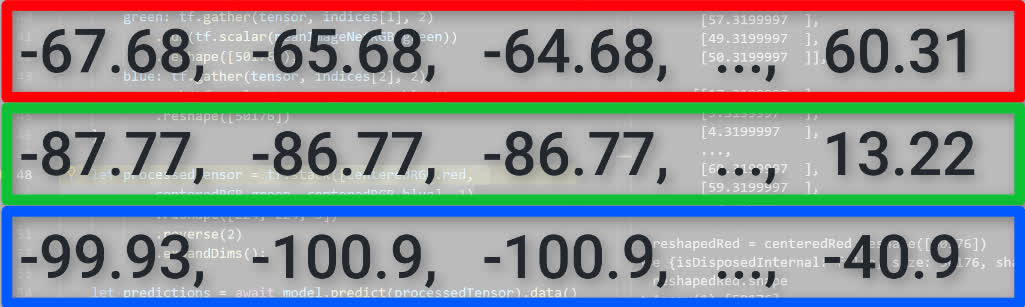
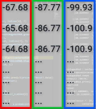
> stackedTensor.print()
Tensor
[[-67.6800003 , -87.7789993 , -99.939003 ],
    [-65.6800003 , -86.7789993 , -100.939003],
    [-64.6800003 , -86.7789993 , -100.939003],
    ...,
    [60.3199997  , 13.2210007  , -42.939003 ],
    [59.3199997  , 12.2210007  , -42.939003 ],
    [60.3199997  , 13.2210007  , -40.939003 ]]
Ok, so we have 50,176 rows each containing a red, green, and blue value.
Now, we need to reshape this guy to be of shape 224 x 224 x 3 before we can pass it to the model, so let's do that with a new variable we'll call reshapedTensor.
> reshapedTensor = stackedTensor.reshape([224, 224, 3])
Ok, let's now print this one.
> reshapedTensor.print()
Tensor
[[[-67.6800003 , -87.7789993 , -99.939003 ],
    [-65.6800003 , -86.7789993 , -100.939003],
    [-64.6800003 , -86.7789993 , -100.939003],
    ...,
    [89.3199997  , 66.2210007  , 59.060997  ],
    [79.3199997  , 53.2210007  , 46.060997  ],
    [66.3199997  , 36.2210007  , 29.060997  ]],

    [[-67.6800003 , -87.7789993 , -99.939003 ],
    [-65.6800003 , -86.7789993 , -100.939003],
    [-64.6800003 , -86.7789993 , -100.939003],
    ...,
    [89.3199997  , 66.2210007  , 59.060997  ],
    [79.3199997  , 53.2210007  , 46.060997  ],
    [66.3199997  , 36.2210007  , 29.060997  ]],

    [[-70.6800003 , -89.7789993 , -98.939003 ],
    [-68.6800003 , -88.7789993 , -99.939003 ],
    [-66.6800003 , -87.7789993 , -99.939003 ],
    ...,
    [85.3199997  , 61.2210007  , 55.060997  ],
    [74.3199997  , 45.2210007  , 38.060997  ],
    [58.3199997  , 26.2210007  , 20.060997  ]],

    ...
    [[22.3199997  , -18.7789993 , -64.939003 ],
    [19.3199997  , -20.7789993 , -63.939003 ],
    [6.3199997   , -30.7789993 , -67.939003 ],
    ...,
    [58.3199997  , 13.2210007  , -39.939003 ],
    [49.3199997  , 6.2210007   , -41.939003 ],
    [50.3199997  , 6.2210007   , -38.939003 ]],

    [[18.3199997  , -22.7789993 , -69.939003 ],
    [15.3199997  , -23.7789993 , -64.939003 ],
    [11.3199997  , -24.7789993 , -60.939003 ],
    ...,
    [57.3199997  , 10.2210007  , -42.939003 ],
    [49.3199997  , 4.2210007   , -48.939003 ],
    [50.3199997  , 5.2210007   , -45.939003 ]],

    [[17.3199997  , -23.7789993 , -65.939003 ],
    [9.3199997   , -29.7789993 , -63.939003 ],
    [4.3199997   , -31.7789993 , -65.939003 ],
    ...,
    [60.3199997  , 13.2210007  , -42.939003 ],
    [59.3199997  , 12.2210007  , -42.939003 ],
    [60.3199997  , 13.2210007  , -40.939003 ]]]
Again, this shape means we have 224 rows each containing 224 pixels, which each contain a red, green, and blue, value.
Then, we need to reverse the values in the tensors along the second axis from RGB to BGR for the reasons we mentioned last time.
So, we'll do that with a new variable, reversedTensor.
> reversedTensor = reshapedTensor.reverse(2)
Let's print this one out.
> reversedTensor.print()
Tensor
[[[-99.939003 , -87.7789993 , -67.6800003 ],
    [-100.939003, -86.7789993 , -65.6800003 ],
    [-100.939003, -86.7789993 , -64.6800003 ],
    ...,
    [59.060997  , 66.2210007  , 89.3199997  ],
    [46.060997  , 53.2210007  , 79.3199997  ],
    [29.060997  , 36.2210007  , 66.3199997  ]],

    [[-99.939003 , -87.7789993 , -67.6800003 ],
    [-100.939003, -86.7789993 , -65.6800003 ],
    [-100.939003, -86.7789993 , -64.6800003 ],
    ...,
    [59.060997  , 66.2210007  , 89.3199997  ],
    [46.060997  , 53.2210007  , 79.3199997  ],
    [29.060997  , 36.2210007  , 66.3199997  ]],

    [[-98.939003 , -89.7789993 , -70.6800003 ],
    [-99.939003 , -88.7789993 , -68.6800003 ],
    [-99.939003 , -87.7789993 , -66.6800003 ],
    ...,
    [55.060997  , 61.2210007  , 85.3199997  ],
    [38.060997  , 45.2210007  , 74.3199997  ],
    [20.060997  , 26.2210007  , 58.3199997  ]],

    ...
    [[-64.939003 , -18.7789993 , 22.3199997  ],
    [-63.939003 , -20.7789993 , 19.3199997  ],
    [-67.939003 , -30.7789993 , 6.3199997   ],
    ...,
    [-39.939003 , 13.2210007  , 58.3199997  ],
    [-41.939003 , 6.2210007   , 49.3199997  ],
    [-38.939003 , 6.2210007   , 50.3199997  ]],

    [[-69.939003 , -22.7789993 , 18.3199997  ],
    [-64.939003 , -23.7789993 , 15.3199997  ],
    [-60.939003 , -24.7789993 , 11.3199997  ],
    ...,
    [-42.939003 , 10.2210007  , 57.3199997  ],
    [-48.939003 , 4.2210007   , 49.3199997  ],
    [-45.939003 , 5.2210007   , 50.3199997  ]],

    [[-65.939003 , -23.7789993 , 17.3199997  ],
    [-63.939003 , -29.7789993 , 9.3199997   ],
    [-65.939003 , -31.7789993 , 4.3199997   ],
    ...,
    [-42.939003 , 13.2210007  , 60.3199997  ],
    [-42.939003 , 12.2210007  , 59.3199997  ],
    [-40.939003 , 13.2210007  , 60.3199997  ]]]
We see the first BGR values we have here are -99, -87, and -76. Let's make sure this is the reverse of the RGB values in our last tensor.
Scrolling up to compare the values in the previous tensor, we can see indeed it is.
Our last operation is expanding the dimensions of our tensor to make it go from a rank-3 tensor to a rank-4 tensor, which is what our model requires.
We create a new variable expandedTensor.
> expandedTensor = reversedTensor.expandDims()
Let's check the shape of this guy.
> expandedTensor.shape
Array(4) [1, 224, 224, 3]
So we have this inserted dimension at the start now, making our tensor rank-4 with shape 1 x 224 x 224 x 3 rather than just 224 x 224 x 3 that we had last time.
Printing this out, we can see this extra dimension added around our previous tensor.
> expandedTensor.print()
Tensor
[[[[-99.939003 , -87.7789993 , -67.6800003 ],
[-100.939003, -86.7789993 , -65.6800003 ],
[-100.939003, -86.7789993 , -64.6800003 ],
...,
[59.060997  , 66.2210007  , 89.3199997  ],
[46.060997  , 53.2210007  , 79.3199997  ],
[29.060997  , 36.2210007  , 66.3199997  ]],

[[-99.939003 , -87.7789993 , -67.6800003 ],
[-100.939003, -86.7789993 , -65.6800003 ],
[-100.939003, -86.7789993 , -64.6800003 ],
...,
[59.060997  , 66.2210007  , 89.3199997  ],
[46.060997  , 53.2210007  , 79.3199997  ],
[29.060997  , 36.2210007  , 66.3199997  ]],

[[-98.939003 , -89.7789993 , -70.6800003 ],
[-99.939003 , -88.7789993 , -68.6800003 ],
[-99.939003 , -87.7789993 , -66.6800003 ],
...,
[55.060997  , 61.2210007  , 85.3199997  ],
[38.060997  , 45.2210007  , 74.3199997  ],
[20.060997  , 26.2210007  , 58.3199997  ]],

...
[[-64.939003 , -18.7789993 , 22.3199997  ],
[-63.939003 , -20.7789993 , 19.3199997  ],
[-67.939003 , -30.7789993 , 6.3199997   ],
...,
[-39.939003 , 13.2210007  , 58.3199997  ],
[-41.939003 , 6.2210007   , 49.3199997  ],
[-38.939003 , 6.2210007   , 50.3199997  ]],

[[-69.939003 , -22.7789993 , 18.3199997  ],
[-64.939003 , -23.7789993 , 15.3199997  ],
[-60.939003 , -24.7789993 , 11.3199997  ],
...,
[-42.939003 , 10.2210007  , 57.3199997  ],
[-48.939003 , 4.2210007   , 49.3199997  ],
[-45.939003 , 5.2210007   , 50.3199997  ]],

[[-65.939003 , -23.7789993 , 17.3199997  ],
[-63.939003 , -29.7789993 , 9.3199997   ],
[-65.939003 , -31.7789993 , 4.3199997   ],
...,
[-42.939003 , 13.2210007  , 60.3199997  ],
[-42.939003 , 12.2210007  , 59.3199997  ],
[-40.939003 , 13.2210007  , 60.3199997  ]]]]
That sums up all of our tensor operations! Quickly though, in case you're not using Visual Studio code, I did want to also show this same set up directly from within the Chrome browser so that you can do your debugging there instead if you'd prefer.
Debugging in Chrome
Opening Chrome, we can right click on the page, click Inspect, and then navigate to the Sources tab. Here, we have access to the source code for our app.
predict.js is currently being shown in the open window, so now we have access to the exact code we were displaying in Visual Studio Code. We can insert breakpoints here in the same way, and
we've placed one on the same line as earlier.
Now let's select an image and click the predict button.
We see that our app is paused at our breakpoint, and then we can step over the code just as we saw earlier as well.
From the Chrome debugger, we also have the ability to view all the variables similar to the Variable panel we saw in Visual Studio Code, and we also have a debugger console where we can run all the same code we ran in Visual Studio Code as well.
Alright, hopefully now, you have a decent grasp on tensors and tensor operations. Let me know what you thought of going through this practice in the debugger to see how the tensors changed over time with each operation, and I'll see ya in the next video.
quiz
 DEEPLIZARD
Message
DEEPLIZARD
Message
resources
updates
Committed by on