TensorFlow - Python Deep Learning Neural Network API

Convolutional neural network predictions with TensorFlow's Keras API

In this episode, we'll demonstrate how to use a convolutional neural network (CNN) for inference to predict on images of cats and dogs using TensorFlow's Keras API.

Last time, we built and trained our very first CNN. We observed that this model performed well on the training set, but didn't do so well generalizing to the validation set. None-the-less, we're now going to see how this model holds up to predicting on images of cats and dogs in our test set.

Given the less-than-decent results we saw from the validation performance, our expectation is that the model likely won't perform any better on the test set. Regardless of the results though, the steps we're about to go through will expose us to the general process for using a CNN for inference.

Preparing the test data

First, ensure that you still have the code in place from last time when we built the model, as well as the earlier episode when we created our test set.

We'll now run next(test_batches) to extract a batch of images and their corresponding labels from the test set.

test_imgs, test_labels = next(test_batches)

Recall, test_batches was created in a previous episode and was created using Keras ImageDataGenerator.flow_from_directory() to generate batches of data from the test set that resides on disk.

Using the plotImages() function we previously introduced, we can see what this batch of test data looks like.

plotImages(test_imgs)
print(test_labels)

[[1. 0.]
 [1. 0.]
 [1. 0.]
 [1. 0.]
 [1. 0.]
 [1. 0.]
 [1. 0.]
 [1. 0.]
 [1. 0.]
 [1. 0.]]

Just as we saw before, cats are labeled with a one-hot encoding of [1,0], and dogs are labeled as [0,1].

Note, because we chose to not shuffle our test set when we originally created it, the first half of the test data is all cats, and the second half is all dogs. Also, recall that the color data appears skewed due to the VGG16 preprocessing we specified when we created the data sets.

Predicting on the test data

Now we'll use our previously built model and call model.predict() to have the model predict on the test set.

predictions = model.predict(x=test_batches, steps=len(test_batches), verbose=0)

We pass in the test set, test_batches, and set steps to be then length of test_batches. Similar to steps_per_epoch that was introduced in the last episode, steps specifies how many batches to yield from the test set before declaring one prediction round complete.

We also specify verbose=0 to see no output during the evaluation process.

After running the predictions, we can print our the rounded predictions see what they look like.

np.round(predictions)

array([[0., 1.],
       [1., 0.],
       [1., 0.],
       [1., 0.],
       [0., 1.],
       ...
])

These are the labels that the model is predicting for our images.

Plotting predictions with a confusion matrix

To get a better visualization of these results, we'll plot them in a confusion matrix, which we've covered in detail in a previous episode.

We create the confusion matrix using scikit-learn, which we imported a couple episodes back.

cm = confusion_matrix(y_true=test_batches.classes, y_pred=np.argmax(predictions, axis=-1))

To the confusion matrix, we pass the true labels of the test set, along with the predicted labels for the test set from the model.

Note, we can access the unshuffled true labels for the test set by calling test_batches.classes.

array([0, 0, 0, 0, 0, 0, 0, 0, 0, 0, 0, 0, 0, 0, 0, 0, 0, 0, 0, 0, 0, 0,
       0, 0, 0, 0, 0, 0, 0, 0, 0, 0, 0, 0, 0, 0, 0, 0, 0, 0, 0, 0, 0, 0,
       0, 0, 0, 0, 0, 0, 1, 1, 1, 1, 1, 1, 1, 1, 1, 1, 1, 1, 1, 1, 1, 1,
       1, 1, 1, 1, 1, 1, 1, 1, 1, 1, 1, 1, 1, 1, 1, 1, 1, 1, 1, 1, 1, 1,
       1, 1, 1, 1, 1, 1, 1, 1, 1, 1, 1, 1
])

We transform the one-hot encoded predicted labels to be in the same format as the true labels by only selecting the element with the highest value for each prediction using np.argmax(predictions, axis=-1).

We then define the plot_confusion_matrix() function that is copied directly from scikit-learn.

def plot_confusion_matrix(cm, classes,
                          normalize=False,
                          title='Confusion matrix',
                          cmap=plt.cm.Blues):
    """
    This function prints and plots the confusion matrix.
    Normalization can be applied by setting `normalize=True`.
    """
    plt.imshow(cm, interpolation='nearest', cmap=cmap)
    plt.title(title)
    plt.colorbar()
    tick_marks = np.arange(len(classes))
    plt.xticks(tick_marks, classes, rotation=45)
    plt.yticks(tick_marks, classes)

    if normalize:
        cm = cm.astype('float') / cm.sum(axis=1)[:, np.newaxis]
        print("Normalized confusion matrix")
    else:
        print('Confusion matrix, without normalization')

    print(cm)

    thresh = cm.max() / 2.
    for i, j in itertools.product(range(cm.shape[0]), range(cm.shape[1])):
        plt.text(j, i, cm[i, j],
            horizontalalignment="center",
            color="white" if cm[i, j] > thresh else "black")

    plt.tight_layout()
    plt.ylabel('True label')
    plt.xlabel('Predicted label')

We can then inspect the class_indices for the labels so that we know in which order to pass them to our confusion matrix.

test_batches.class_indices

{'cat': 0, 'dog': 1}

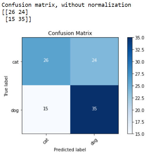
Finally, we plot the confusion matrix.

cm_plot_labels = ['cat','dog']
plot_confusion_matrix(cm=cm, classes=cm_plot_labels, title='Confusion Matrix')

We can see that the model correctly predicted that an image was a cat 26 times when it actually was a cat, and it incorrectly predicted that an image was a cat 15 times when it was not a cat. It correctly predicted that an image was a dog 35 times, and incorrectly predicted that an image was a dog 24 times.

Given what we saw last time from the validation metrics, these results are not surprising.

Now that we have a general understanding for how to build and work with a CNN using Keras, we'll now move on to working with a pre-trained model on this data set, which we will see will generalize much better!