
Max Pooling in Convolutional Neural Networks explained
text
Max Pooling in Convolutional Neural Networks
Hey, what's going on everyone? In this post, we're going to discuss what max pooling is in a convolutional neural network. Without further ado, let's get started.

We're going to start out by explaining what max pooling is, and we'll show how it's calculated by looking at some examples. We'll then discuss the motivation for why max pooling is used, and we'll see how we can add max pooling to a convolutional neural network in code using Keras.
We're going to be building on some of the ideas that we discussed in our post on CNNs, so if you haven't seen that yet, go ahead and check it out, and then come back to read this post once you've finished up there.
Introducing max pooling
Max pooling is a type of operation that is typically added to CNNs following individual convolutional layers.
When added to a model, max pooling reduces the dimensionality of images by reducing the number of pixels in the output from the previous convolutional layer.
Let's go ahead and check out a couple of examples to see what exactly max pooling is doing operation-wise, and then we'll come back to discuss why we may want to use max pooling.
Example using a sample from the MNIST dataset
We've seen in our post on CNNs that each convolutional layer has some number of filters that we define with a specified dimension and that these filters convolve our image input channels.
When a filter convolves a given input, it then gives us an output. This output is a matrix of pixels with the values that were computed during the convolutions that occurred on our image. We call these output channels.
We're going to be using the same image of a seven that we used in our previous post on CNNs. Recall, we have a matrix of the pixel values from an image of a 7 from the MNIST data set.
We used a 3 x 3 filter to produce the output channel below:
| 0.0 | 0.0 | 0.0 | 0.0 | 0.0 | 0.0 | 0.0 | 0.0 | 0.0 | 0.0 | 0.0 | 0.0 | 0.0 | 0.0 | 0.0 | 0.0 | 0.0 | 0.0 | 0.0 | 0.0 | 0.0 | 0.0 | 0.0 | 0.0 | 0.0 | 0.0 |
| 0.0 | 0.0 | 0.0 | 0.0 | 0.0 | 0.0 | 0.0 | 0.0 | 0.0 | 0.0 | 0.0 | 0.0 | 0.0 | 0.0 | 0.0 | 0.0 | 0.0 | 0.0 | 0.0 | 0.0 | 0.0 | 0.0 | 0.0 | 0.0 | 0.0 | 0.0 |
| 0.0 | 0.0 | 0.0 | 0.0 | 0.0 | 0.0 | 0.0 | 0.0 | 0.0 | 0.0 | 0.0 | 0.0 | 0.0 | 0.0 | 0.0 | 0.0 | 0.0 | 0.0 | 0.0 | 0.0 | 0.0 | 0.0 | 0.0 | 0.0 | 0.0 | 0.0 |
| 0.0 | 0.0 | 0.0 | 0.0 | 0.0 | 0.0 | 0.0 | 0.0 | 0.0 | 0.0 | 0.0 | 0.0 | 0.0 | 0.0 | 0.0 | 0.0 | 0.0 | 0.0 | 0.0 | 0.0 | 0.0 | 0.0 | 0.0 | 0.0 | 0.0 | 0.0 |
| 0.0 | 0.0 | 0.0 | 0.0 | 0.0 | 0.0 | 0.0 | 0.0 | 0.0 | 0.0 | 0.0 | 0.0 | 0.0 | 0.0 | 0.0 | 0.0 | 0.0 | 0.0 | 0.0 | 0.0 | 0.0 | 0.0 | 0.0 | 0.0 | 0.0 | 0.0 |
| 0.0 | 0.0 | 0.0 | 0.0 | 0.0 | 0.0 | 0.0 | 0.0 | 0.0 | 0.3 | 0.4 | 0.6 | 0.7 | 0.5 | 0.4 | 0.1 | 0.0 | 0.0 | 0.0 | 0.0 | 0.0 | 0.0 | 0.0 | 0.0 | 0.0 | 0.0 |
| 0.0 | 0.3 | 0.6 | 1.2 | 1.4 | 1.6 | 1.6 | 1.6 | 1.6 | 1.9 | 1.9 | 2.2 | 2.3 | 2.1 | 2.0 | 1.7 | 0.9 | 0.5 | 0.0 | 0.0 | 0.0 | 0.0 | 0.0 | 0.0 | 0.0 | 0.0 |
| 0.5 | 1.2 | 1.8 | 2.6 | 2.7 | 3.0 | 3.0 | 3.0 | 3.0 | 3.4 | 3.5 | 3.8 | 4.0 | 3.7 | 3.6 | 3.2 | 2.3 | 1.5 | 0.5 | 0.1 | 0.0 | 0.0 | 0.0 | 0.0 | 0.0 | 0.0 |
| 1.1 | 2.1 | 3.2 | 4.2 | 4.4 | 4.7 | 4.7 | 4.5 | 4.2 | 4.0 | 3.8 | 3.9 | 3.9 | 4.1 | 4.5 | 4.7 | 4.1 | 3.1 | 1.5 | 0.5 | 0.0 | 0.0 | 0.0 | 0.0 | 0.0 | 0.0 |
| 1.1 | 2.0 | 3.1 | 3.6 | 3.3 | 3.2 | 3.2 | 3.1 | 2.9 | 2.7 | 2.5 | 2.5 | 2.5 | 2.7 | 3.0 | 3.9 | 4.4 | 4.1 | 2.9 | 1.4 | 0.3 | 0.0 | 0.0 | 0.0 | 0.0 | 0.0 |
| 0.9 | 1.4 | 2.1 | 2.2 | 1.8 | 1.7 | 1.7 | 1.5 | 1.1 | 0.8 | 0.5 | 0.5 | 0.5 | 0.8 | 1.3 | 2.4 | 3.7 | 4.5 | 4.0 | 2.4 | 1.0 | 0.0 | 0.0 | 0.0 | 0.0 | 0.0 |
| 0.1 | 0.3 | 0.3 | 0.3 | 0.0 | 0.0 | 0.0 | 0.0 | 0.0 | 0.0 | 0.0 | 0.0 | 0.0 | 0.0 | 0.1 | 1.3 | 2.8 | 4.2 | 4.7 | 2.8 | 1.6 | 0.0 | 0.0 | 0.0 | 0.0 | 0.0 |
| 0.0 | 0.0 | 0.0 | 0.0 | 0.0 | 0.0 | 0.0 | 0.0 | 0.0 | 0.0 | 0.0 | 0.0 | 0.0 | 0.0 | 0.4 | 1.2 | 2.9 | 3.9 | 5.1 | 3.1 | 2.2 | 0.1 | 0.0 | 0.0 | 0.0 | 0.0 |
| 0.0 | 0.0 | 0.0 | 0.0 | 0.0 | 0.0 | 0.0 | 0.0 | 0.0 | 0.1 | 0.4 | 1.0 | 1.3 | 1.6 | 1.9 | 2.4 | 3.7 | 4.4 | 5.2 | 3.8 | 2.5 | 0.7 | 0.0 | 0.0 | 0.0 | 0.0 |
| 0.0 | 0.0 | 0.0 | 0.0 | 0.0 | 0.0 | 0.0 | 0.2 | 0.5 | 1.1 | 1.7 | 2.3 | 2.7 | 3.0 | 3.4 | 3.7 | 4.6 | 4.9 | 5.2 | 4.1 | 2.5 | 1.2 | 0.0 | 0.0 | 0.0 | 0.0 |
| 0.0 | 0.0 | 0.0 | 0.0 | 0.0 | 0.1 | 0.7 | 1.3 | 1.9 | 2.6 | 3.2 | 4.0 | 4.4 | 4.8 | 4.4 | 4.2 | 4.5 | 4.8 | 5.2 | 4.5 | 2.7 | 1.6 | 0.0 | 0.0 | 0.0 | 0.0 |
| 0.0 | 0.0 | 0.0 | 0.0 | 0.4 | 1.0 | 1.8 | 2.6 | 3.3 | 3.8 | 3.9 | 3.8 | 3.6 | 3.4 | 3.0 | 2.9 | 3.6 | 4.1 | 5.0 | 3.8 | 2.5 | 1.0 | 0.0 | 0.0 | 0.0 | 0.0 |
| 0.0 | 0.0 | 0.0 | 0.0 | 0.8 | 1.7 | 3.0 | 3.5 | 3.7 | 3.3 | 3.0 | 2.5 | 2.2 | 1.9 | 1.3 | 1.3 | 2.4 | 3.3 | 4.8 | 3.4 | 2.3 | 0.6 | 0.0 | 0.0 | 0.0 | 0.0 |
| 0.0 | 0.0 | 0.0 | 0.0 | 0.9 | 2.0 | 2.7 | 3.2 | 2.6 | 1.8 | 1.3 | 0.7 | 0.4 | 0.1 | 0.0 | 0.4 | 2.2 | 3.3 | 4.6 | 3.0 | 2.0 | 0.2 | 0.0 | 0.0 | 0.0 | 0.0 |
| 0.0 | 0.0 | 0.0 | 0.0 | 0.7 | 1.4 | 1.6 | 1.7 | 0.7 | 0.2 | 0.0 | 0.0 | 0.0 | 0.0 | 0.0 | 0.8 | 2.5 | 3.7 | 4.2 | 2.6 | 1.5 | 0.0 | 0.0 | 0.0 | 0.0 | 0.0 |
| 0.0 | 0.0 | 0.0 | 0.0 | 0.1 | 0.5 | 0.2 | 0.5 | 0.0 | 0.0 | 0.0 | 0.0 | 0.0 | 0.0 | 0.7 | 1.7 | 3.3 | 4.0 | 3.6 | 2.2 | 0.8 | 0.0 | 0.0 | 0.0 | 0.0 | 0.0 |
| 0.0 | 0.0 | 0.0 | 0.0 | 0.0 | 0.0 | 0.0 | 0.0 | 0.0 | 0.0 | 0.0 | 0.0 | 0.0 | 0.0 | 1.3 | 2.3 | 4.0 | 3.9 | 2.8 | 1.6 | 0.2 | 0.0 | 0.0 | 0.0 | 0.0 | 0.0 |
| 0.0 | 0.0 | 0.0 | 0.0 | 0.0 | 0.0 | 0.0 | 0.0 | 0.0 | 0.0 | 0.0 | 0.0 | 0.0 | 0.3 | 2.3 | 3.1 | 4.5 | 3.4 | 2.0 | 0.8 | 0.0 | 0.0 | 0.0 | 0.0 | 0.0 | 0.0 |
| 0.0 | 0.0 | 0.0 | 0.0 | 0.0 | 0.0 | 0.0 | 0.0 | 0.0 | 0.0 | 0.0 | 0.0 | 0.0 | 0.9 | 2.6 | 3.4 | 3.8 | 2.5 | 1.2 | 0.2 | 0.0 | 0.0 | 0.0 | 0.0 | 0.0 | 0.0 |
| 0.0 | 0.0 | 0.0 | 0.0 | 0.0 | 0.0 | 0.0 | 0.0 | 0.0 | 0.0 | 0.0 | 0.0 | 0.0 | 1.2 | 2.0 | 2.8 | 2.4 | 1.5 | 0.3 | 0.0 | 0.0 | 0.0 | 0.0 | 0.0 | 0.0 | 0.0 |
| 0.0 | 0.0 | 0.0 | 0.0 | 0.0 | 0.0 | 0.0 | 0.0 | 0.0 | 0.0 | 0.0 | 0.0 | 0.0 | 1.0 | 1.3 | 2.0 | 1.3 | 0.6 | 0.0 | 0.0 | 0.0 | 0.0 | 0.0 | 0.0 | 0.0 | 0.0 |
As mentioned earlier, max pooling is added after a convolutional layer. This is the output from the convolution operation and is the input to the max pooling operation.
After the max pooling operation, we have the following output channel:
| 0.0 | 0.0 | 0.0 | 0.0 | 0.0 | 0.0 | 0.0 | 0.0 | 0.0 | 0.0 | 0.0 | 0.0 | 0.0 |
| 0.0 | 0.0 | 0.0 | 0.0 | 0.0 | 0.0 | 0.0 | 0.0 | 0.0 | 0.0 | 0.0 | 0.0 | 0.0 |
| 0.0 | 0.0 | 0.0 | 0.0 | 0.3 | 0.6 | 0.7 | 0.4 | 0.0 | 0.0 | 0.0 | 0.0 | 0.0 |
| 1.2 | 2.6 | 3.0 | 3.0 | 3.4 | 3.8 | 4.0 | 3.6 | 2.3 | 0.5 | 0.0 | 0.0 | 0.0 |
| 2.1 | 4.2 | 4.7 | 4.7 | 4.2 | 3.9 | 4.1 | 4.7 | 4.4 | 2.9 | 0.3 | 0.0 | 0.0 |
| 1.4 | 2.2 | 1.8 | 1.7 | 1.1 | 0.5 | 0.8 | 2.4 | 4.5 | 4.7 | 1.6 | 0.0 | 0.0 |
| 0.0 | 0.0 | 0.0 | 0.0 | 0.1 | 1.0 | 1.6 | 2.4 | 4.4 | 5.2 | 2.5 | 0.0 | 0.0 |
| 0.0 | 0.0 | 0.1 | 1.3 | 2.6 | 4.0 | 4.8 | 4.4 | 4.9 | 5.2 | 2.7 | 0.0 | 0.0 |
| 0.0 | 0.0 | 1.7 | 3.5 | 3.8 | 3.9 | 3.6 | 3.0 | 4.1 | 5.0 | 2.5 | 0.0 | 0.0 |
| 0.0 | 0.0 | 2.0 | 3.2 | 2.6 | 1.3 | 0.4 | 0.8 | 3.7 | 4.6 | 2.0 | 0.0 | 0.0 |
| 0.0 | 0.0 | 0.5 | 0.5 | 0.0 | 0.0 | 0.0 | 2.3 | 4.0 | 3.6 | 0.8 | 0.0 | 0.0 |
| 0.0 | 0.0 | 0.0 | 0.0 | 0.0 | 0.0 | 0.9 | 3.4 | 4.5 | 2.0 | 0.0 | 0.0 | 0.0 |
| 0.0 | 0.0 | 0.0 | 0.0 | 0.0 | 0.0 | 1.2 | 2.8 | 2.4 | 0.3 | 0.0 | 0.0 | 0.0 |
Max pooling works like this. We define some n x n region as a corresponding filter for the max pooling operation. We're going to use 2 x 2 in this example.
We define a stride, which determines how many pixels we want our filter to move as it slides across the image.
Stride determines how many units the filter slides.
On the convolutional output, and we take the first 2 x 2 region and calculate the max value from each value in the 2 x 2 block. This value is stored in the output channel, which
makes up the full output from this max pooling operation.
We move over by the number of pixels that we defined our stride size to be. We're using 2 here, so we just slide over by 2, then do the same thing. We calculate the max value
in the next
2 x 2 block, store it in the output, and then, go on our way sliding over by 2 again.
Once we reach the edge over on the far right, we then move down by 2 (because that's our stride size), and then we do the same exact thing of calculating the max value for the
2 x 2 blocks in this row.
We can think of these 2 x 2 blocks as
pools of numbers, and since we're taking the max value from each pool, we can see where the name
max pooling came from.
This process is carried out for the entire image, and when we're finished, we get the new representation of the image, the output channel.
In this example, our convolution operation output is 26 x 26 in size. After performing max pooling, we can see the dimension of this image was reduced by a factor of 2 and is now
13 x 13.
Just to make sure we fully understand this operation, we're going to quickly look at a scaled down example that may be more simple to visualize.
Scaled down example
Suppose we have the following:
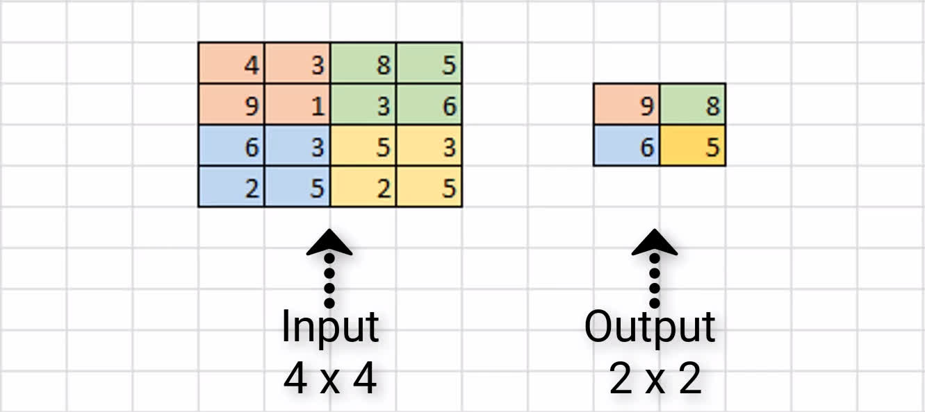
We have some sample input of size 4 x 4, and we're assuming that we have a 2 x 2 filter size with a stride of 2 to do max pooling on this input channel.
Our first 2 x 2 region is in orange, and we can see the max value of this region is 9, and so we store that over in the output channel.
Next, we slide over by 2 pixels, and we see the max value in the green region is 8. As a result, we store the value over in the output channel.
Since we've reached the edge, we now move back over to the far left, and go down by 2 pixels. Here, the max value in the blue region is 6, and we store that here in our output
channel.
Finally, we move to the right by 2, and see the max value of the yellow region is 5. We store this value in our output channel.
This completes the process of max pooling on this sample 4 x 4 input channel, and the resulting output channel is this 2 x 2 block. As a result, we can see that our input dimensions
were again reduced by a factor of two.
Alright, we know what max pooling is and how it works, so let's discuss why would we want to add this to our network?
Why use max pooling?
There are a couple of reasons why adding max pooling to our network may be helpful.
Reducing computational load
Since max pooling is reducing the resolution of the given output of a convolutional layer, the network will be looking at larger areas of the image at a time going forward, which reduces the amount of parameters in the network and consequently reduces computational load.
Reducing overfitting
Additionally, max pooling may also help to reduce overfitting. The intuition for why max pooling works is that, for a particular image, our network will be looking to extract some particular features.
Maybe, it's trying to identify numbers from the MNIST dataset, and so it's looking for edges, and curves, and circles, and such. From the output of the convolutional layer, we can think of the higher valued pixels as being the ones that are the most activated.
With max pooling, as we're going over each region from the convolutional output, we're able to pick out the most activated pixels and preserve these high values going forward while discarding the lower valued pixels that are not as activated.
Just to mention quickly before going forward, there are other types of pooling that follow the exact same process we've just gone through, except for that it does some other operation on the regions rather than finding the max value.
Average pooling
For example, average pooling is another type of pooling, and that's where you take the average value from each region rather than the max.
Currently max pooling is used vastly more than average pooling, but I did just want to mention that point. Alright, now let's jump over to Keras and see how this is done in code.
Working with code in Keras
We'll start with some imports:import keras
from keras.models import Sequential
from keras.layers import Activation
from keras.layers.core import Dense, Flatten
from keras.layers.convolutional import *
from keras.layers.pooling import *
Here, we have a completely arbitrary CNN.
model_valid = Sequential([
    Dense(16, input_shape=(20,20,3), activation='relu'),
    Conv2D(32, kernel_size=(3,3), activation='relu', padding='same'),
    MaxPooling2D(pool_size=(2, 2), strides=2, padding='valid'),
    Conv2D(64, kernel_size=(5,5), activation='relu', padding='same'),
    Flatten(),
    Dense(2, activation='softmax')
])
It has an input layer that accepts input of 20 x 20 x 3 dimensions, then a dense layer followed by a convolutional layer followed by a max pooling layer, and then one more convolutional layer, which
is finally followed by an output layer.
Following the first convolutional layer, we specify max pooling. Since the convolutional layers are 2d here, We're using the MaxPooling2D layer from Keras, but Keras also has
1d and 3d max pooling layers as well.
The first parameter we're specifying is the pool_size. This is the size of what we were calling a filter before, and in our example, we used a 2 x 2 filter.
The next parameter is strides. Again, in our earlier examples, we used 2 as well, so that's what we've specified here. The last parameter that we have specified is the
padding parameter. If you're unsure what
padding or zero-padding is in regards to CNNs, be sure to check out the earlier post that explains the concept.
Recall from that post, we discussed how valid padding means to use no padding, that's what we've specified here, and actually I don't think it's a common practice at all to use padding on max pooling layers.
But while we're on the subject of padding, I wanted to point something else out, which is that for the two convolutional layers, we've specified same padding so that the input is padded such that the output of the convolutional layers will be the same size as the input.
If we go ahead and look at a summary of our model, we can see that the dimensions from the output of our first layer are 20 x 20, which matches the original input size. The dimensions of the output
from our first convolutional layer maintain the same 20 x 20 values because we're using same padding on that layer.
> model_valid.summary()

_________________________________________________________________
Layer (type)                 Output Shape              Param #
=================================================================
dense_2 (Dense)              (None, 20, 20, 16)        64
_________________________________________________________________
conv2d_1 (Conv2D)            (None, 20, 20, 32)        4640
_________________________________________________________________
max_pooling2d_1 (MaxPooling2 (None, 10, 10, 32)        0
_________________________________________________________________
conv2d_2 (Conv2D)            (None, 10, 10, 64)        51264
_________________________________________________________________
flatten_1 (Flatten)          (None, 6400)              0
_________________________________________________________________
dense_2 (Dense)              (None, 2)                 12802
=================================================================
Total params: 68,770
Trainable params: 68,770
Non-trainable params: 0
_________________________________________________________________
Once we go down to the max pooling layer, we see the value of the dimensions has been cut in half to become 10 x 10. This is because, as we saw with our earlier examples, a filter of size
2 x 2 along with a stride of 2 for our max pooling layer will reduce the dimensions of our input by a factor of two, so that's exactly what we see here.
Lastly, this max pooling layer is followed by one last convolutional layer that is using same padding, so we can see that the output shape for this last layer maintains the 10 x 10 dimensions from
the previous max pooling layer.
Wrapping up
At this point, we should have gained an understanding for what max pooling is, what it achieves when we add it to a CNN, and how we can specify max pooling in your own network using Keras. I'll see ya next time!
quiz
 DEEPLIZARD
Message
DEEPLIZARD
Message
resources
updates
Committed by on