Neural Network Programming - Deep Learning with PyTorch

Neural Network Batch Processing with PyTorch

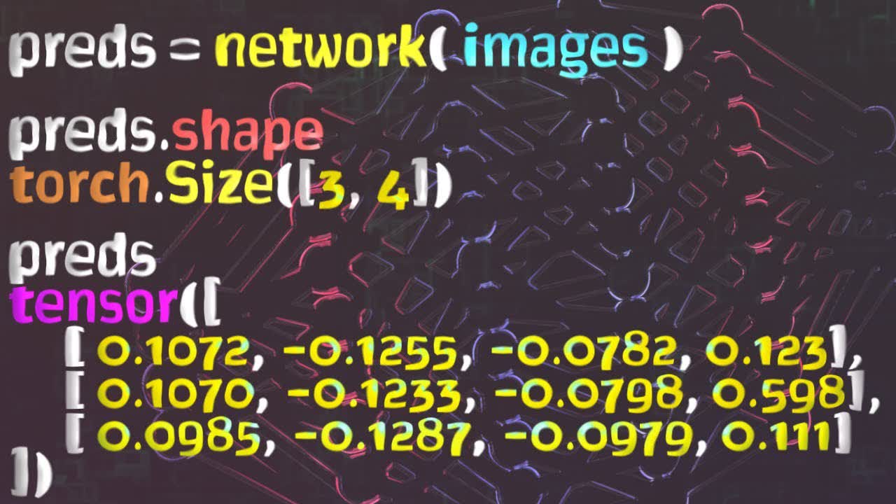
Welcome to this neural network programming series with PyTorch. Our goal in this episode is to pass a batch of images to our network and interpret the results. Without further ado, let's get started.

• Prepare the data
• Build the model
  • Understand how batches are passed to the network
• Train the model
• Analyze the model’s results

In the last episode, we learned about forward propagation and how to pass a single image from our training set to our network. Now, let's see how to do this using a batch of images. We'll use the data loader to get the batch, and then, after passing the batch to the network, we'll interpret the output.

Passing a Batch of Images to the Network

Let’s begin by reviewing the code setup from the last episode. We need the following:

1. Our imports.
2. Our training set.
3. Our Network class definition.
4. To disable gradient tracking. (optional)
5. A Network class instance.

Now, we’ll use our training set to create a new DataLoader instance, and we’ll set our batch_size=10, so the outputs will be more manageable.

> data_loader = torch.utils.data.DataLoader(
     train_set, batch_size=10
)

We’ll pull a batch from the data loader and unpack the image and label tensors from the batch. We’ll name our variables using the plural forms since we know the data loader is returning a batch of ten images when we call next on the data loader iterator.

> batch = next(iter(data_loader))
> images, labels = batch

This gives us two tensors, a tensor of images and a tensor of corresponding labels.

In the last episode, when we pulled a single image from our training set, we had to unsqueeze() the tensor to add another dimension that would effectively transform the singleton image into a batch with a size of one. Now that we are working with the data loader, we are dealing with batches by default, so there is no further processing needed.

The data loader returns a batch of images that are packaged into a single tensor with a shape that reflects the following axes.

This means tensor's shape is in good shape, and there's no need to unsqueeze it. ;)

> images.shape
torch.Size([10, 1, 28, 28])

> labels.shape
torch.Size([10])

Let's interpret both of these shapes. The first axis of the image tensor tells us that we have a batch of ten images. These ten images have a single color channel with a height and width of twenty-eight.

The labels tensor has a single axis with a shape of ten, which corresponds to the ten images inside our batch. One label for each image.

Alright. Let’s get a prediction by passing the images tensor to the network.

> preds = network(images)

> preds.shape
torch.Size([10, 10])

> preds
tensor(
    [
        [ 0.1072, -0.1255, -0.0782, -0.1073,  0.1048,  0.1142, -0.0804, -0.0087,  0.0082,  0.0180],
        [ 0.1070, -0.1233, -0.0798, -0.1060,  0.1065,  0.1163, -0.0689, -0.0142,  0.0085,  0.0134],
        [ 0.0985, -0.1287, -0.0979, -0.1001,  0.1092,  0.1129, -0.0605, -0.0248,  0.0290,  0.0066],
        [ 0.0989, -0.1295, -0.0944, -0.1054,  0.1071,  0.1146, -0.0596, -0.0249,  0.0273,  0.0059],
        [ 0.1004, -0.1273, -0.0843, -0.1127,  0.1072,  0.1183, -0.0670, -0.0162,  0.0129,  0.0101],
        [ 0.1036, -0.1245, -0.0842, -0.1047,  0.1097,  0.1176, -0.0682, -0.0126,  0.0128,  0.0147],
        [ 0.1093, -0.1292, -0.0961, -0.1006,  0.1106,  0.1096, -0.0633, -0.0163,  0.0215,  0.0046],
        [ 0.1026, -0.1204, -0.0799, -0.1060,  0.1077,  0.1207, -0.0741, -0.0124,  0.0098,  0.0202],
        [ 0.0991, -0.1275, -0.0911, -0.0980,  0.1109,  0.1134, -0.0625, -0.0391,  0.0318,  0.0104],
        [ 0.1007, -0.1212, -0.0918, -0.0962,  0.1168,  0.1105, -0.0719, -0.0265,  0.0207,  0.0157]
    ]
)

The prediction tensor has a shape of 10 by 10, which gives us two axes that each have a length of ten. This reflects the fact that we have ten images and for each of these ten images we have ten prediction classes.

The elements of the first dimension are arrays of length ten. Each of these array elements contain the ten predictions for each category for the corresponding image.

The elements of the second dimension are numbers. Each number is the assigned value of the specific output class. The output classes are encoded by the indexes, so each index represents a specific output class. This mapping is given by this table.

Fashion MNIST Classes

Using Argmax: Prediction vs Label

To check the predictions against the labels, we use the argmax() function to figure out which index contains the highest prediction value. Once we know which index has the highest prediction value, we can compare the index with the label to see if there is a match.

To do this, we call the argmax() function on the prediction tensor, and we specify second dimension.

The second dimension is the last dimension of our prediction tensor. Remember from all of our work on tensors, the last dimension of a tensor always contains numbers while every other dimension contains other smaller tensor.

In our prediction tensor's case, we have ten groups of numbers. What the argmax() function is doing is looking inside each of these ten groups, finding the max value, and outputting its index.

For each group of ten numbers:
1. Find max value.
2. Output index

The interpretation of this is that, for each of the images in the batch, we are finding the prediction class that has the highest value. This is the category the network is predicting most strongly.

> preds.argmax(dim=1)
tensor([5, 5, 5, 5, 5, 5, 4, 5, 5, 4])

> labels
tensor([9, 0, 0, 3, 0, 2, 7, 2, 5, 5])

The result from the argmax() function is a tensor of ten prediction categories. Each number is the index where the highest value occurred. We have ten numbers because there were ten images. Once we have this tensor of indices of highest values, we can compare it against the label tensor.

> preds.argmax(dim=1).eq(labels)
tensor(
[False, False, False, False, False, False, False, False, True, False]
)

> preds.argmax(dim=1).eq(labels).sum()
tensor(1)

To achieve the comparison, we are using the eq() function. The eq() function computes an element-wise equals operation between the argmax output and the labels tensor.

This returns True if the prediction category in the argmax output matches the label and False otherwise.

Finally, if we call the sum() function on this result, we can reduce the output into a single number of correct predictions inside this scalar valued tensor.

We can wrap this last call into a function called get_num_correct() that accepts the predictions and the labels, and uses the item() method to return the Python number of correct predictions.

def get_num_correct(preds, labels):
    return preds.argmax(dim=1).eq(labels).sum().item()

Calling this function, we can see we get the value 1.

> get_num_correct(preds, labels)
1

Conclusion

We should now have a good understanding of how to pass a batch of inputs to a network and what the expected shape is when dealing with a convolutional neural network.

I’ll see you in the next one.